Basic Graduate Evolution
Table of Contents
- Notes
- Review genetic basics
- More genetic basics
- Dynamics of Genes in Populations
- Dynamics of Genes in Populations
- Population Size and Neutral Theory
- Rates and Patterns of Nucleotide Substitution
- Rates and Patterns of Nucleotide Substitution
- Patterns of substitution
- Polymorphism
- C-value paradox
- Gene Evolution
- –Missed Class–
- Inbreeding
- Fixation Index or F-Statistics
- Inbreeding Population Subdivision and Migration
- Second Half
- Phenotypic Plasticity and GxE interactions
- Correlations among traits
- Genetic Variation (book notes)
- QTL Mapping
- Lets play with R
- –Missed Class–
- Natural Selection (book notes)
- Natural Selection 2
- Agents of natural selection
- Evolution of Senescence
- Phylogenetics
- Learn the mesqite software package
- Phylogenetics II
- Downstream uses of Phylogenies
- Community Phylogenetics
- Terms
Notes
Review genetic basics
DNA and RNA
nucleotide ≅ base
Bases
- purines (A T), 3 H bonds, less stable (fewer bonds)
- pyrimidine (GC), 3 H bonds
| RNA | normally single stranded |
| DNA | double stranded |
Each strand has a 5' end and a 3' end. The convention is to write from the 5' and to the 3' end when transcribing DNA. The strands are anti-parallel.
RNA (as compared to DNA)
- single stranded
- much shorter (often 20-24 nucleotides long)
- Bases: (A C G U)
Genes
- traditionally, something that codes for a protein, i.e., gene → messenger-RNA → protein (this was previously the only functionality known for DNA segments)
- now, genes also include sequences which do other things, e.g., transcribe RNA, some RNA sequences are functional as themselves
Types of Genes
- protein coding
- RNA
- regularity
Eukaryotic protein coding genes comprise both transcribed () and non-transcribed () parts.
Gene's are transcribed by polymerase, which first anchors to a "promoter region" which flanks the gene, and then travels the gene transcribing its contents.
A "codon" is 3 nucleatides which are transcribed into 1 amino-acid.
Gene Structure (we're talking about protein coding gene)
- TATA box
- in the promoter region -19 from the gene start, in a GC-rich region of the DNA. Not required, but prevalent
A Gene with the promoter region.
  promoter region       Gene->
---->  --  <---  --     ----------   --------   ---------
GC    CAAT   GC  TATA
box    box  box  box
RNA polymerase
| I | RNA |
| II | protein coding |
| III | small RNA |
- Genes specifying proteins
Transcription and Translation process
- DNA -> pre-RNA (which does include non-coding introns)
- pre-RNA -> mature mRNA, this is done by the spicing machinery (these arose early in evolution and are very intricate machines). Genes are spliced using the "GT-AT rule" (introns often start with GT and end with AG)
- Mature mRNA -> the remainder of the gene is split up into codons and transcribed, it must start with one of three start codons (UGA UAA UAG). The start code does not code for an amino acid. This is still capped by small untranslated sections on either side.
- Protein -> only the translated regions converted to amino acids
There are many other regulatory sequences in introns or between genes which do things like increase or decrease the speed of translation.
- RNA-specifying genes (transcribed to RNA, not translated to protein)
- transfer RNA
- ribosomal RNA
- similar sequences between (eukaryotes and prokaryotes) which means they arose early and are important
Degenerate genetic code
- 20 Amino Acids
- 64 codons (4 × 4 × 4)
- Regulatory Genes
- regulate the expression of another gene
- not transcribed or translated
enhancers or repressors (change tempo of translation)
notable examples
- replicator genes
- initialize and terminate replication
- telomeres
- "cap" at the end of a chromosomes, these erode with age, these don't erode as quickly in sea turtles
- segregator genes
- help split the DNA pair (sisters) for translation, this is where the zippers attach to unzip
- recombination genes
- sites for recombination during meiosis (crossover more likely to happen here)
Amino Acids
Composed of
- a central carbon
- an amino end
- a carboxyl end
- a hydrogen
- a side chain – this is the most variable and the most important
Simplest is glycine
- single H side chain
- fits in nooks and crannies of proteins
Five classes
- positively charged
- negatively charged
- hydrophobic
- neutral
- special
Protein
string of amino acid
- secondary structure – two most common 2-D structures for folded proteins
- α helix
- β pleated sheet
- tertiary structure – these combine into 3-D structures of the protein
- quartinary structure – two tertiary molecules
More genetic basics
phase
Losing the phase (correct codon alignment) can be caused by mutations and garbles the translation resulting in a garbled protein. The phase is determined by the start or initiation codon, and is called the "reading frame" or "open reading frame" (ORF).
degeneracy
Genetic code is degenerate but not ambiguous.
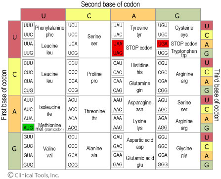
Multiple codons coding for an amino acid will often differ in the third position.
Terminology
- fourfold-degenerate site
- any nucleotide in this position will specify the same amino acid.
- twofold-degenerate site
- two of the four nucleotides at this position will specify the same amino acid.
- non-degenerate site
- every nucleotide here results in a different amino acid, called an "amino-acid substitution".
- synonymous codons
- different codons which code for the same amino acid.
In most codons the first two positions are non-degenerate sites.
numbers of codons
- 61 sense codons (remaining 3 are STOP codons)
- 549 possible codon nucleotide substitutions
- 61 codons × 3 positions × (4-1) alternatives for each position
- assuming equally probable mutations (not true), then 70% of all 3^{rd} position changes are synonymous
- 2^{nd} site is the most sensitive to substitution, 0% of changes are synonymous
- in the 1^{st} site only 4% of changes are synonymous
Main evolutionary forces (on populations)
- mutation
- selection
- migration (new alleles from outside)
- drift
mutations
Mutations are hereditary changes in the genetic material due to errors in DNA replication or DNA repair.
Types of mutations
- substitutions
- recombination (crossing-over and gene conversion)
- deletions/insertions ("indels")
- duplication
- inversions
Evolutionarily mutations that occur in germ cells are the only hereditary ones.
- classes of mutations
- substitutions
also called "point mutations"
classifications
- transitions (purine to purine, pyrimidine to pyrimidine), there
are four possibilities for this
- a ↔ g
- t ↔ c
- transversions change the type, there are eight possibilities for this
If these were equally likely you would expect twice as many transversions as compared to transitions.
You actually see many more transitions than translations.
Also classified by effect (only applies to protein coding genes)
- silent or synonymous (no amino acid change)
- replacement or non-synonymous (cause aa change)
- missense (now codes a new aa)
- nonsense (changes to a termination codon, will prematurely terminate translation)
- transitions (purine to purine, pyrimidine to pyrimidine), there
are four possibilities for this
- crossing-over and gene conversion
- homologous recombination
- occurs between strands which are similar through a shared common ancestry
This happens most often during repair. Say a chromosome breaks (very common) there is a machine which comes along and repairs the broken chromosome (sometimes this causes a change).
This also happens during meiosis.
Two types of homologous recombination
- crossing over (reciprocal recombination), two chromosomes pair up and each gets a bit of the other
- gene-conversion (nonreciprocal recombination), a bit of one goes to another, but one remains unchanged
- insertions and deletions
- unequal crossing over
- May be caused by unequal crossing over,
this is often caused by similar sub-sequences, this could cause
an insertion and a deletion. Generally 10-13 nucleotides long.
-----=====----- ------------- x ---------======----- -----====---====------ - replication slippage
- (look up in a text book), when a repeating pattern is offset. These can be thousands of base pairs long
- retro-transposition
- Selfish elements which are prone to copy themselves anywhere throughout the genome (discovered by Barbara McKlintoc in corn). Sometimes these elements will grab a nearby section of the sequence and bring them along.
- inversion
A rotation of a double-stranded segment by 180.
 |     |
a b c d e f g h
   to
a d c b e f g h
These often occur between genes where they don't have much effect.
- substitutions
- spatial distribution of mutation
Often 100-fold differences in mutation rates between elements of the sequence. These are often very repetitive sequences of the genome.
Some groups of nucleotides are prone to change. E.g.,
CGis easily methelated causing the C to become a T.TTis also a hot spot.palindromes
epigenetics (non-genetic), e.g., chemical elements changing genetic interpretations.
- chemicals inhibiting expression
- proteins binding up DNA into little balls, by histomes, this inhibits transcription
- substitution in non-coding sequences and pseudo-genes
important to determine the pattern of spontaneous mutation
no selective pressure
mutation accumulation experiments, you maintain the lowest possible population size
you could bottleneck a population, no selection, only genetic drift
Pseudo-genes are dead (premature STOP or something), these can also indicate baseline rates.
- can compare to an active duplicate
- can compare to a homolog (inactive in people, compared to active in chimps)
Trend from GC to AT, so non-coding regions become
AT-rich.
Dynamics of Genes in Populations
- Q
- Why does population size matter?
- A
- Selection does not work in small populations.
Evolution as a population-level process
Big "macro-level" changes (e.g., between species) are results of the same small "micro-level" changes between individuals.
Four major evolutionary forces
- mutation
- random genetic drift – ∃! animal, the Atlantic eel, which has an effectively infinite population size, because they all come together to one place annually to mate.
- natural selection
- gene flow
The study of gene changes in populations is population genetics.
- what influences mutant allele over time
- how is genetic variability maintained
- probability of going to fixation
- how fast will replacement take place
- influence of chance effects on molecular genetic change
Definitions
(see Terms)
locus, allele, allele frequencies, genotype, phenotype, discrete trait, continuous or quantitative trait, homozygous vs. heterozygous, genotypic vs. phenotypic ratios, dominant vs. recessive allele, evolution, natural selection, fitness (w)
Punnett Square
- BB is homozygous
- Bb is heterozygous
Mendel bred purple × purple plants and got both purple and white plants. Specifically 705 purple and 224 white.
Diploid parent will produce single-ploid gametes (else there would be a combinatorial explosion in the ploidy of the offspring).
A Punnett Square
| pollen | |||
|---|---|---|---|
| B | b | ||
| pistil | B | BB (purple) | Bb (purple) |
| b | Bb (purple) | bb (purple) |
- phenotypic ratio of above is
- 3 purple
- 1 white
- genotypic ratio of above is
- 1 BB
- 2 Bb
- 1 bb
Changes in allele frequencies
Problem
- 1000 peppered moths in Manchester
- dark melanic form of allele is dominant (M)
- ancestral is recessive (m)
- 825 melanic
- 175 peppered
- 512 of melanic are heterozygous
Some calculations
- Phenotypic ratio is 875/175 or 4.7 melanic to peppered
- Genotypic ratio is 313 MM, 512 Mm, 175 mm or 1.78 : 2.93 : 1
- Allele frequencies of M and m 616 + 512 / 2000 = 0.569 (2 * 175) + 512 / 2000 = 0.431
Allele frequencies are changed by
- selection
- drift
- migration
2 Mathematical approaches
- deterministic
- (analytic) can predict changes unambiguously. The first of these was "Harvey Weinberg".
- stochastic
- probabilistic, associates probability distributions with environmental conditions
Deterministic assumptions
- infinite population size
- constant environment
Needed for Darwinian selection (influenced by Menthusian principles)
- variation
- environmental limit to population size (carry capacity)
- differential reproduction (because of the above)
Types of mutation
     +------------ mutation ------------------+
     |                  |                     |
     |                  |                     |
     |                  |                     |
deleterious          neutral            advantageous
     |                  |                     |
     |                  |                     |
     |                  |                     |
     |                  |                     |
purifying            chance             positive selection
selection            events                   or
                                         overdominant
                                          selection
Normally selection reduces genetic variation, however "overdominant" selection can increase genetic variation. This is when the heterozygote has the highest fitness.
Hardy-Weinberg principle
1 locus, 2 alleles (A_{1} A_{2})
- 3 possibly diploid genotypes
- allelic frequencies are
- f(A_{1}) = p
- f(A_{2}) = q
- p + q = 1
| genotype | A1 A1 | A1 A2 | A2 A2 |
|---|---|---|---|
| p * p | 2pq | q * q |
genotypic frequencies
- f(A_{1}) = p^{2}
- f(A_{2}) = 2pq
- p + q = q^{2}
This is the null model.
Back to our problem.
- melanic is dominant and is 87% (could be heterozygotes)
- → 13% is non-melanic
- → q = 0.13
- → q = \sqrt{0.13} = 0.36
- → p = 1 - q = 0.64
- → f(Mm) = 2pq = 2 × 0.36 × 0.64
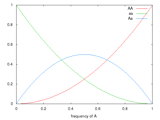
Graph (frequency of a, by frequency of genotype in population)
set xrange [0:1]
set xlabel 'frequency of A'
plot x * x title 'AA', (1-x) * (1-x) title 'aa', 2 * x * (1-x) title 'Aa'
Natural Selection changes allelic frequencies
| genotype | A1 A1 | A1 A2 | A2 A2 |
|---|---|---|---|
| fitness | w11 | w12 | w22 |
| frequency | |||
| after | p * p w11 | 2pqw12 | q * q * w22 |
| selection |
change in frequency
\begin{equation*} \delta q = q' - q \end{equation*} \begin{equation*} \delta q = \frac{pq(p(w_{12} - w_{11}) + q(w_{22} - w_{12}))}{p^{2}w_{11} + 2pqw_{12} + q^{2}w_{22}} \end{equation*}Example
- heterozygous individuals have lighter eye spots (increased predation)
- relative fitness of genotypes
SS 1 Ss 0.9 ss 0.6 - p(S) = 0.7
p = 0.7 q = 0.3
Frequencies in the original
| p | 0.49 |
| pq | 0.09 |
| q | 0.42 |
Relative fitness
| p | 1 |
| pq | 0.9 |
| q | 0.6 |
Next generation frequencies
- f(SS)' = p^{2}w_{11} = 0.49 × 1
- f(Ss)' = 2pqw_{12} = 0.42 × 0.9
- f(ss)' = q^{2}w_{22} = 0.09 × 0.6
Next generation's allelic frequencies
- f(SS) × 2 + f(Ss)
- f(ss) × 2 + f(Ss)
Dynamics of Genes in Populations
Selection is limited in that it can't reduce global population fitness, so drift is essential to navigate landscapes with valleys.
changing allele frequencies with overdominance
- Overdominance is also called heterozygote superiority.
- When the heterozygote has a higher fitness than either homozygote.
- this is one of the few times (along with frequency dependent selection) in which selection increases genetic diversity
- called "balancing" or "stabilizing" selection
The equilibrium frequency (\(\hat{p}\)) is given by
\begin{equation*} \hat{p} = \frac{w_{12}- w_{22}}{2w_{12} - w_{11} - w_{22}} \end{equation*}When w11=0.9, w12=1, and w22=0.8 then \(\hat{p} = 0.667\).
\(\bar{w}\) is the average fitness of the entire population.
Examples of Overdominant Selection – Sickle-cell Anemia
"find them and grind them" ← experimental identification of overdominant selection. Cavalli-Sforza is prolific in this area.
| type | codon | amino-acid | cell shape |
|---|---|---|---|
| wild type | GAG |
glu | doughnut |
| mutant | GTG |
val | cycle |
The wild type allele is more dominance, but it is not a perfect dominance relation.
| alleles | anemia | malaria | fitness |
|---|---|---|---|
| SS | normal | vulnerable | 0.9 |
| Ss | slight | resistant | 1.0 |
| ss | severe | 0.2 |
Underdominance
This is an unstable equilibrium, any deviation from equilibrium will fall away.
This is another instance of a valley which selection can not traverse.
Drift
- Changes in allele frequency due solely to chance effects.
- Moral is not to assume that every trait is adaptive.
- Especially important in our currently world of many species with severely reduced population sizes. Note: this will reduce the likelihood that these populations will be able to adapt to climate change.
Stochastic events from ecology have huge effects on small populations.
- alley effect
- catastrophe
;; the above generated with the following
(loop :for pop-size :in '(100000 1000000) :do
   (with-open-file (out (format nil "/tmp/pop~d.data" pop-size) :direction :output)
     (gen-drift out :pop-size pop-size)))
Wright-Fisher model of random genetic drift
- depiction of the sampling process in populations of finite size
- the distribution of frequencies of gametes is expected to follow a binomial distribution
Process
- N individuals in P_{0}produce ∞ gametes
- 2N gametes are selected from the pool of ∞ gametes
- N individuals in P_{1}
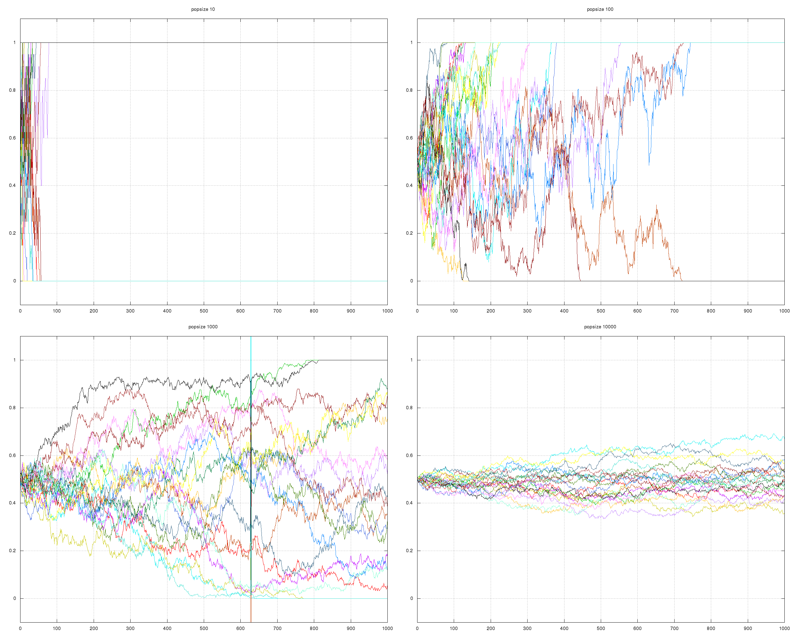
Consider a diploid population of N individuals w/2N genes
when 2N gametes are sampled from the ∞ gamete pool the probability P_{i} of i genes of type A is given by
\begin{equation*} P_{i} = \frac{(2N)!}{i! (2N-i)!} p^{i}q^{2N-i} \end{equation*}Make some graphs of a population of a given size with some number of genes, should the frequency of each gene over a number of generations to show the increased effect of chance in smaller populations.
Pea pod
A pot of 100 seeds, 50 round and 50 wrinkled.
Enumerate all possible samples and the related probability of such a sample.
- Probability of four round seeds = \(\frac{4!}{4! 0!} 0.5^{4} 0.5^{0} = 2^{-4}\)
- Probability of three round seeds = \(\frac{4!}{3! 1!} 0.5^{3} 0.5^{1} = 4 \times 2^{-3} \times 2^{-1}\)
- Probability of two of each = \(\frac{4!}{2! 2!} 0.5^{2} 0.5^{2} = 4 \times 2^{-2} \times 2^{-2}\)
Population Size and Neutral Theory
Wright-Fisher model of random genetic drift
N individuals → ∞ gametes → N individuals → ∞ gametes
\begin{equation*} P_{i} = \frac{(2N)!}{i! (2N-i)!} p^{i}q^{2N-i} \end{equation*}For an idealized population and makes the following assumptions
- all individuals contribute gametes equally to the next generation
- population size is constant
- non-overlapping generations
effective population size
N_{e}: The size of an idealized population which would have the same effect of random sampling on gene frequency as that in the actual population.
N: The observed actual population size (census size).
Generally N_{e} << N, or roughly \(\frac{N}{3}\), because of
- Pre- and post-reproductive individuals should not be counted.
- difference in ratio of males to females, in which case \begin{eqnarray*} N_{e} &=& \frac{4N_{m}N_{f}}{N_{m}+N_{f}}, where\\ N_{m} &=& \text{num males}\\ N_{f} &=& \text{num females} \end{eqnarray*}
Also due to long-term variations in pop-size
- environmental catastrophes
- cyclical model of reproduction
- local extinction and re-colonization events
The long term size is the harmonic mean of population sizes (where n is the number of generations). Thus dips in population size affect the long term size more than temporary peaks.
\begin{equation*} N_{e} = \frac{n}{(\frac{1}{N_{1}} + \frac{1}{N_{2}} + \ldots + \frac{1}{N_{n}})} \end{equation*}Long bottlenecks have much more of an impact on maintained genetic diversity than short bottlenecks. It is impressive how much variation may be maintained even through very narrow short bottlenecks.
gene substitution and related topics (definitions)
- gene substitution
- the process whereby a mutant allele completely replace the predominant or wild-type allele in the population
- fixation time
- time (usually measured in # generations) it takes for a mutant allele to become fixed in a population
- fixation probability
- the chance that a new mutant allele will reach fixation in a population
- rate of gene substitution
- number of substitutions or fixations per unit time
fixation probability
- fixation probability determined by
- initial frequency (often 1/2N)
- selective advantage
- the effective population size N_{e} ← very important
Fitness for an allele is equal to a combination of S and N_{e}
- Selection coefficient (S) or (w - S)
S=0 neutral S>0 beneficial S<0 deleterious - in small populations basically everything is neutral
P probability of fixating
- neutral
- \(p = \frac{1}{2N}\)
- small selection coefficients
- \(P = \frac{2s}{(1 - e^{-4Ns})}\)
- positive values of s and large N
- P = 2s
- example of fixation probability
- N_{e} = 1000 = N
- a new mutant arises
so initial frequency = 1/2000
- let this new mutant be neutral, so s = 0
then probability of fixation P = 1/2000.
- with a slight selective advantage, e.g., s=0.01
then P = \frac{2s}{(1 - e^{-4Ns})} ≅ 2s = 0.02
- with a slight selective disadvantage, e.g., s=-0.001
then P = \frac{2s}{(1 - e^{-4Ns})} ≅ 2s = 3.7314723e-5
(defun adv (s N) (/ (* 2 s) (- 1 (exp (* -4 N s)))))
fixation time
the time required for fixation or loss of a neutral allele depends upon
- initial frequency
- population size N
times shorten as frequency approaches 1 or 0
For a new mutation (Kimura and Ohta 1969) with initial frequency 1/2N, the mean time to fixation is ≈
- neutral allele
- \(\bar{t} = 4N generations\)
- allele with a selective advantage of S
- \(\bar{t} = \frac{2}{s}\ln{\left(\frac{2}{N}\right)}\)
- example (lets say a mouse)
- N_{e} = 10^{6}
- generation time = 2 years
For a neutral mutant allele in will take 4N = 4(10^{6}) = 8 mil. years.
For a slightly selective allele (s=0.01)
\frac{2}{0.01} × ln{(2/N)} = 5,800 years
gene substitutions (neutral mutations)
Rate of gene substitutions (reaching fixations) per unit time.
neutral mutations
- neutral mutation rate = μ per gene per generation
- number of mutations arising at a locus in a diploid pop of size N = 2Nμ per generation
- but the probability of fixation of each mutation is P = 1/2N
Therefore the substitution rate is
K = (number of mutations)(probability of fixation)
or
\begin{equation*} K = 2 N \mu P = (2N\mu)(1/2N) = \mu \end{equation*}substitution rate = mutation rate (thanks Kimura)
gene substitutions (advantageous mutations)
- advantageous mutation rate μ per gene per generation
- mutations per locus is 2Nμ per generation
- probability of fixation is P=2s
therefore
K = (num of mutations) (probability of fixation) (selection coefficient)
\begin{equation*} K = 2N\mu P = (2N\mu)(2s) = 4Ns\mu \end{equation*}getting started with neutral theory
Rates and patterns of nucleotide substitutions, and molecular clock.
Darwin didn't know the mechanisms of heredity.
Mendel was treated as a crackpot because most people studied bio-metric continuous quantitative traits with normal distributions. So Mendel went back to gardening.
New-Darwinian theory Darwin and Mendel combined.
- mutation ultimate source of genetic variation
- natural selection given the dominant "creative" role in shaping genetic make-up of populations
Selectionism
- natural selection only evolutionary force
- polymorphism must be maintained by balancing selection
- gene substitution must be due to selection of advantageous mutations
Rates and Patterns of Nucleotide Substitution
Neutral Theory of Molecular Evolution
- Gelatin pheresis?
- Finding large amounts of genetic variability in natural populations.
- how to explain this in terms of selection
- Fisher promoted eugenics.
- Haldane. 1960s ← awesome wild man
The selective death that must occur for a gene to be substituted over another allele.
Thus if all genetic variation was due to selection, this would require more death than the populations could tolerate
- calculated upper limit of 1 gene substitution per 300 generations
read the following papers
- The Cost of Selection Haldane 1954, Journal of Genetics
- Our load of mutations Muller HJ 1950, American Journal of Human Genetics
- Number of alleles that can be maintained in a finite population Kimura and Crow 1964, Genetics 49:725
Beginning of the neutral theory,
The Neutral Theory of Mutation Kimura 1968
most polymorphisms observed at the molecular level are selectively neutral, so that their frequency dynamics in a population are determined by random genetic drift.
Selection can not account for the following, drift can
- Haldane's cost of selection – rate of change of amino-acids in haemoglobin over time, it was changing too fast to be selective, ~1000 fold over Haldane's limit
- segregational load, when the most fit genotype is a heterozygote (overdominance). In combination with Mendelian Segregation ensures that in each generation inferior homozygous combinations will be produced. The segregational load is the decrease in population fitness due to these homozygotes. This load would be unbearable if all heterozygotes were selective.
Theoretical Principles of the Neutral Theory
Models the fate of selectively neutral (neutral or nearly neutral) mutations through drift.
- The probability of fixation of a neutral allele in a population equals its frequency P_{0}.
- The steady-state rate at which neutral mutations are fixed in a population equals the neutral mutation rate μ. Fixation is new mutations × probability of fixation. \begin{equation*} P_{fixation} = (2N\mu) \times (\frac{1}{2N}) = \mu \end{equation*}
- Average time between neutral substitutions is \(\frac{1}{\mu}\).
- New neutral mutations destined to be fixed require on average \(4N_{e}\) generations to come to fixation. Newly arising neutral mutations destined to be lost require on average \(\frac{2N_{e}}{N}\ln{2N}\)
- If each neutral mutation creates a new universally unique allele,
then at equilibrium, the average number of new alleles gained
through mutation is exactly offset by the average number lost by
genetic drift. At this point the amount of expected homozygosity
equals
\begin{equation*}
\frac{1}{\theta+1}=\frac{1}{4N_{e}\mu + 1}
\end{equation*}
because
\begin{equation*} \theta=4N_{e}\mu \end{equation*}- equilibrium average homozygosity = 1/(1+θ)
- equilibrium average heterozygosity = θ/(1+θ)
This is one of the first parameters you'll measure when finding a new population in the wild. Heterozygosity → genetic variation → evolvability. From this you can infer bottlenecks in the evolutionary history of the population.
Excessive heterozygosity can be an indication that two previously isolated populations have recently mixed.
More heterozygosity in larger populations.
Estimating rates of molecular sequence divergence
mechanisms of substitution can be elucidated by comparing substitution rates among
- genes
- different DNA regions of genes
- non-coding regions of the genome
Knowing the rate of nucleotide substitution may also enable us to date evolutionary events (e.g., divergence between species).
How variable is the rate of change between different evolutionary lineages? Is there a universal evolutionary clock? Definitely different for different genes and portions of DNA.
              /--- xxoxoxxxxx
 ancestral   /
xxxxxxxxxx --  total evolutionary time = 2t
 sequence    \
              \--- xxxxxoxxxx
            time t
- L
- total number of sites (10 here)
- \(\hat{D}\)
- proportion of sites that differ in the two sequences (3/10 here)
Formulas
- for relatively short intervals of evolutionary time, we can use \(\hat{D}\) (proportion of differences) in estimating the rate of molecular evolution
- over long periods of time the sequences becomes so saturated that multiple hits cannot be identified.
- \(\hat{K}\) takes these multiple hits into account
\begin{equation*}
\hat{K} = -\ln{(1-\hat{D})}
\end{equation*}
for nucleotides
\begin{equation*} \hat{k} = -(\frac{3}{4}) ln (1-(\frac{4}{3}\hat{d})) \end{equation*} - estimated rate of evolution \begin{equation*} \hat{\lambda} = \frac{\hat{K}}{s\hat{t}} \end{equation*}
Write out \hat{\lambda} as amino acid replacement per amino-acid site per year.
Rates and Patterns of Nucleotide Substitution
Estimated rates of molecular sequence divergence
- amino acids called replacements
- nucleotides called substitutions
Rates of nucleotide substitution
- Rates of substitution complicated by cases in which different nucleotides mutation to being the same.
- several models of nucleotide substitution, differ primarily in rates of mutation between nucleotides
- simplest model is "Jukes Cantor" (all probabilities are equal)
Jukes-Cantor model
- L = length of sequence
- \hat{d} = proportion of sites that differ in the sequences
- \(\hat{k} = (\frac{3}{4})\ln{(1-4\frac{\hat{d}}{3})}\)
- \(\hat{\lambda} = \frac{\hat{k}}{2\hat{t}}\)
Kimura 2-parameter model
- 4 transitions possible and 8 transversions possible
- in the data despite numbers there were many more transitions than transversions
- updates the Jukes-Cantor model with two transition rates α and β depending on if the mutation is a transition or a transversion
- example
trpA divergence for amino acids
- 20 amino acids
- 2 are different so
- \(\hat{d} = 0.1\)
- \(\hat{k} = 0.105\)
- \(\hat{\lambda} = 0.105/(2 \times 80 million years) = 0.66 \times 10^{-9}\) per site per mil years
(log (- 1 (* 0.1))) ;; => -0.105360545
trpA divergence for nucleotides
- 60 places
- 9 differing sites
- \(\hat{d} = 9/60\)
- \(\hat{k} = -3/4 ln(1-4/3\times\hat{d}) = 0.167\)
- \(\hat{\lambda} = 0.167/(2 \times 80 million years) = 1.04\times10^{-9}/site/year\)
Molecular Clock
The rate of mutation is surprisingly constant
The notion of the "Molecular Clock" was first attributed to Emile Zuckerkandi and Linus Pauling.
- across different times
- across different species
- across all genes
Used by Kimura as evidence of neutral molecular evolution.
Variation in the rate of the molecular clock
- neutral mutation rate << overall mutation rate
- neutral mutation rate may vary widely across genes. Some genes are strongly conserved (e.g., histones) and some vary quickly (e.g., immunity with diversity at a premium – in fact humans pick mates with different genetic material at immune sites, leads to children with diverse immune system.).
- pattern of hereditary transmission leads to variable rates
- mitochondrial DNA is very fast in animals
- mitochondrial DNA is very slow in plants
- X-linked genes have slow mutation rate than autosomal genes
- substitution rates can also vary across sites within genes
Molecular Clock in Genes Varies Directly with the Neutral Mutation Rates
Genes have different neutral mutation rates depending on how well they are conserved.
Find graph of (corrected amino acid changes /100 residues) by millions of years since divergence.
Molecular evolution in the NS genes of influenza virus.
Rates vary widely! e.g., 10^{-9} for some organisms, but as high as 10^{-3} for some RNA viruses (RNA does not have a good proof-reading mechanism – but they don't mind as they evolve out from under our vaccines).
HIV started spreading in the 1920s in Africa caused by colonialism (see the book Tinderbox), had been in rural Africa for a long time, but was constrained by small village sizes.
Does the constancy of substitution rates prove the neutral theory
- it would seem so
- a perfectly driven molecular clock driven by a random process should have a Poisson distribution (variance = mean)
- analysis of substitution rates for different genes for pairs of
species violated Poisson expectations
- perfect clock, variation in rate of ticking = average rate of ticking
- Poisson, prob of a number of events in a fixed period of time (assumes events occur independently at some average rate)
- in three different studies the Var >> Mean
- the excess variance in substitution rates has been called an "Episodic Clock", characterized by periods of stasis alternating with periods of rapid substitution
| var >> mean | clumped |
| var ~= mean | constant |
| var << mean | too evenly distributed (not independent) |
Patterns of substitution
- patterns of substitutions for coding regions
- synonymous/silent substitutions
- non-synonymous/replacement substitutions
4-fold degenerate sites
- TCN → ser
2-fold degenerate sites
- CAY → His y=any pyrmidine
- CAR → Gln R=any purine
Total # synonymous sites:
- # of 4-fold degenerate sites + 1/3 (# of 2-fold deererate sites)
Total # non-synonymous sites:
- # of non-degenerate sites + 2/3 (# of 2-fold deererate sites)
\(\frac{K_{A}}{k_{S}} = \frac{d_{N}}{d_{S}}\) → tells you the amt. of selective constraints on a gene
- if \(\frac{K_{A}}{k_{S}}=1\) then neutral
- if \(\frac{K_{A}}{k_{S}}<1\) then purifying selection
- if \(\frac{K_{A}}{k_{S}}>1\) positive selection
Neutral Theory predicts that the rate of the molecular clock should run at different rates of different organisms having different neutral mutation rates
- RAN virus polymerase lacks effective proofreading mechanisms
Expected rate of substitution of neutral alleles equals the rate of mutation μ to neutral alleles
- Poisson distribution (variance=mean)
Perfect clock: variance in rate of ticking = rate of mutation
Analysis of substitution rates: violated
- var >> mean → clumped
- var == mean → Poisson
- var << mean → evenly distributed
Polymorphism
Drosophila Example
Drosophila adh gene (breaks down alcohol in rotting fruit)
- 3 adh alleles
- differ at 5 positions along 2379 base pairs
- nucleotide polymorphism ps=5/2379
- π calculation:
- 3 alleles, 3 pairwise comparisons (\(\frac{n \times (n-1)}{2}\))
- Ja-S(1)
- Ja-s(2)
- F1-F
- 3 alleles, 3 pairwise comparisons (\(\frac{n \times (n-1)}{2}\))
Heterozygosity
- Ja-S(1) vs. Ja-s(2) = 0 ← (should be different: problem w/problem)
- Ja-S(1) vs. F1-F = 5/2379
- Ja-S(2) vs. F1-F = 5/2379
- average per site (or nucleotide diversity in the sample) = π = 10/(3×2379)
Polymorphism under Neutral Expectations
- divergence
- inter-specific, between species
- polymorphism
- intra-specific, within species
Both driven by the neutral mutation rate. So these should co-vary.
Hudson-Kreitman-Aguade (HKA) Test
- Neutral Theory predicts both
- the rates of substitution over time
- the amount of polymorphism within a population
- Both of these are determined by the mutation rate of the gene
- Given this the HKA test detects natural selection
- two different genetic regions in at least two different species
- calculation of both within-species variation and between-species divergence
- expected values of above are a function of
- time t since divergence
- the relative effective population sizes
- the θ=4N_{e}μ value for each gene
HKA Test application (Maze Teosinte)
Two genetic regions relating to gene tb 1
- 5' regulatory non-transcribed NTR region
- coding region of tb 1
     |
 wild| -----              mutation rate along DNA region
     |      \--\          between maize and wild teosinte
     |          \
     |           \-
     |             \
   μ |              \
     |               \
     |                \-
maize| ------------------\
     |                   --------------------
     |
     +---------------------------------------
                      DNA
        non-coding            coding
95% reduction in variation in maize in this NTR region for maze as compared to teosinte (p=0.004).
McDonald-Kreitman Test (1993)
This is limited to coding region because of the synonymous/non-synonymous bit.
- simpler statistical test to detect natural selection at the sequence level (compared to HKA test)
- Based on the same fundamental principles for non-synonymous (replacement) and synonymous (silent) changes in the coding region of a gene
- if observed substitutions are neutral, then non-synonymous to synonymous ration between species should equal the ratio within species
McDonald-Kreitman Test in Drosophila
- 42 silent and 2 replacement changes within D. melanogaster
- 17 silent and 7 replacement changes between D. melanogaster and two other species
differences
- Fixed difference are between species
- polymorphic differences are intra-species
| fixed | polymorphism | totals | expected fixed | expected poly | crit exp | crit poly | |
|---|---|---|---|---|---|---|---|
| replacement | 7 | 2 | 9 | 3.1764706 | 5.8235294 | 4.6023965 | 2.5103981 |
| silent | 17 | 42 | 59 | 20.823529 | 38.176471 | 0.70206035 | 0.38294200 |
| totals | 24 | 44 | 68 | ||||
| ratio | 0.70833333 | 0.95454545 | 0.86764706 |
From the total ratio (0.867…) we can calculate the expected replacement/silent for fixed/polymorphism. We can then compare these expected values to the observed using a Χ^{2} test.
Note: The most powerful test for selection.
We have a df=1 with a p<0.01, we reject the null of neutral evolution, and know there is purifying selection within D. melanogaster.
Genome Sizes
Smallest known genome (non-viral): Bacterium Carsonella ruddii 160,000 base pairs; an endosymbiont, with 182 genes.
~500 minimum genes to be free living
Smallest genome for free-living organism: Bacterium Mycoplasma genitalium – 580,ooo base pairs (probably ~500 genes)
Largest known Genome: Amoeba Amoeba dubia – 670,000,000,000 base pairs
~115 million-fold difference!
Genome Sizes and Gene Number
find this graph
Smaller genomes fit close to the 100% coding line, then around 10^3 Megabases we start to see the % coding drops off and we have more junk DNA (small RNAs, regulatory stuff etc…).
Genome size is the amount of DNA in the Haploid gene (sperm or egg). This is commonly called the c-value.
- Larger genomes generally measured in pico-grams (pg) of DNA.
- Smaller genomes generally measured in base pairs or kilo-base-pairs
Among bacteria, 20-fold range in number of genes and 20-fold range in genome size, do not appear to contain large quantities of nongenetic DNA. Three fractions
- chromosomal
- protein coding 70-80%, spacers RNA 20-30%, RNA 1%
- plasmid-derived
- extra chromosomal and genes
- transposable
- common components, insertion sequences (more junky)
C-value paradox
Genome Sizes of Bacteria
Explanation of distribution in genome size in bacteria
- major and minor peaks in the genome size of bacteria, these relate to gene duplication, and they all appear to have happened at roughly the same time (around the time when the atmosphere switched largely to oxygen)
- these genome duplication's occurred independently in many lineages
- small scale insertions and deletions
- duplicative transposition
- horizontal transfer of genes, derived mainly from plasmids
- loss of massive chunks of DNA in many parasitic lines
Genome sizes in Eukaryotes
some (birds) have little variability, others (e.g., amoebas) have huge ranges (e.g., ~20,000 fold).
no real correlation between size and complexity
even some sister species have huge differences in genome sizes
- 20-fold range in number of genes
- 80,000-fold range in the size of the genome
non-genetic DNA is left of the sole culprit in the C-value paradox
The Precambrian Radiation
most growth through duplication
Types of gene duplication
- partial gene
- whole gene
- single chromosome
- whole genome
Genes Populations
- Genes duplicate with great frequency
- it is possible to study genes using population models
- get a gene
- find all instances of it in a set of DNA
- use k_{S} to compare the relative ages and times since duplication
- use cohort analysis to find the typical ages of the genes
The duplication of genes is a primary driver of genetic evolution!
Gene Evolution
Looking at age distribution of duplicate-genes, generally an L-shaped distribution with many young duplicates and much fewer old duplicates.
mechanisms of small-scale gene duplication
- unequal crossing-over
- retro-transposition, a transposon moves and takes a gene with it
- fragment capture by double strand break
                               2 regulatory    coding
                              --====---===---============--

                                        | duplication
                                        v

                              --xxxx---===---============--
                              --====---===---============--

                                new     | degeneration
                                 |      v
                                 v
                              --xxxx---===---============--
                              --====---===---============--

                                     complementation

--xxxx---===---============-- --====---===---============-- --====--knocked out========--
--====---xxx---============-- --====---YYY---============-- --====---===---============--
    sub-functionalization          neo-functionalization        non-functionalization
   (both needed to retain          (a new function after          (most common, one
    ancestoral function)              mutation)                     is just worthless)
after duplication one element is free to adapt to a new purpose without losing the functionality of the original
Canonical model for Evolution of Functionally Novel Proteins
Ohno 1970
- complete gene duplication, regulatory and coding portions. one of these copies will stay under selection, the other will be free to drift
- either neo-functionalization or non-functionalization, often that
later occasionally the former
- point mutations
- short insertions and deletions
Example Evolution of tri-chromatic Vision in Ohno's Model (tinkering)
by Opsin gene duplication in Old World Primates
- gene duplication leading to red and blue ~500 Million years ago (using K_{s})
- splits (some monkeys still only have red and blue)
- in our line there is a red duplication, one of these duplicates evolves into a green sensor (15/348 sites have amino acid substitution)
Example Evolution Freezing Avoidance (large change)
- Arctic fish evolved their own antifreeze proteins, which bind to tiny ice crystals and prevent them from forming larger pieces of ice
- this novel anti-freeze gene was a partial duplication of a pancreatic (digestive) enzyme
- the small first exon is duplicated along with the first intron, and half of the second exon. 9 base pairs straddling the beginning of the second exon, are duplicated again and again and again forming a very large exon. This is "internal amplification".
Radically new functions often the product of moving around large chunks of a gene not through point mutations.
Chimeric Genes – Creation of Novel Genes by Exon shuffling
- TPA is derived from four genes
- TPA is a unique protein not found elsewhere, it protects red blood cells by breaking down blood clots and allows signaling between organs/tissues
Many exons code for functionality independent "domains" of a protein.
The TPA protein has 4 exons coming from 3 different genes.
This process is called "exon shuffling".
Frequent Convergent Evolution
- evolution of hermaphrodism in 2 of many species of little worms
- parsimonious solution would be that it only evolved once, actual solution is convergent evolution
–Missed Class–
Inbreeding
Inbreeding increases homozygosity and decreases heterozygosity.
This depends upon both the duration of inbreeding and the closeness of the inbreeding pairs.
levels of closeness
- self-fertilization
- full-sib mating
- double first-cousin mating
   1 | ---\-----
     |  \\-     \-----
     |  |  \          \-----     3
heter|   \  \               \----
ozygo|   |   \                   \-----
sity |    \   \-                       \-----
     |     \    \                            \--
     |     |     ----    2
     |      \        \-------
     |      |   1            \------
     |       ---                    \---
     |          \----
   0 +---------------\-------------------------
           5           10          15         20
                  Generations
full self'ing will lose heterozygosity by half every generation
Genetic Consequences of Inbreeding
- Inbreeding does not alter allele frequency, p/q stays the same.
- Inbreeding does push heterozygotes to homozygotes
- relative to Hardy Weinberg frequencies
- F = inbreeding coefficient
- H_{i} = (2pq - 2pqF) = prob gene in an inbred individual I is heterozygous
- H_{s} = proportion of heterozygous genotypes expected in random mating
- F_{is} = proportion reduction in heterozygotes due to inbreeding relative to the subpopulation as a whole \begin{equation*} F_{is} = \frac{H_{s} - H_{i}}{H_{s}} = \frac{2pq - (2pq - 2pqF)}{2pq} = F \end{equation*}
- Inbreeding with natural selection can change allele frequencies
through "Inbreeding Depression"
- inbreeding depression has been shown for a long time in both laboratory and domesticated populations
- most populations carry deleterious recessive alleles at low frequency at many loci, many of these are recessive and heterozygous
- inbreeding makes many of these harmful recessive alleles homozygous, exposing their harmful effects to natural selection
- Inbreeding can increase "Linkage Disequilibrium"
- lets take loci 1 and 2, with alleles Aa and Bb respectively.
- linkage disequilibrium exists if certain combinations (say AB and ab) are represented in gametes more frequently than by chance and other (say Ab and aB) are less than by chance.
Population Subdivision or Structure
- organisms rarely exist as a single panmictic population in nature
- naturally aggregate in flocks, herds, colonies, schools, prides
- genetic differentiation is inevitable in these cases
- independent aggregate effects of mutation, natural selection and random drift
- this can lead to speciation
- gene flow among populations via migration slows this divergence
In population genetics migration is often treated in the same way as mutation. Just a new allele in the population.
Walhund Effect
the reduction in heterozygosity in a population caused by subpopulation structure
- sometimes subdivision and isolation in nature are not obvious (e.g.,
D pseudoobscura and D. persimilis overlap in distribution)
- they are subpopulations with limited gene-flow between them
- moral: don't trust morphology to differentiate species, use genetics
- example
- consider a population that is subdivided into two subpopulations of equal size
- random intra-population mating, but not between
- sample 100 individuals from each
genotype A1A1 A1A2 A2A2 sub-pop 1 64 32 4 sub-pop 2 4 32 64 total 68 64 68 The total looks to be Hardy-Weinberg, but isolated sub-populations are definately not Hardy-Weinberg.
Assume that the sub-pops match Hardy-Weinberg distributions.
- in that case the expected frequency of heterozygotes would be 0.5
- the actual frequency of heterozygotes is 0.32
- this is not underdominance, this is the "Walhund Effect"
Heirarchical Population Structure
nested subpopulations
stream < river < watershed < continent
F statistics
- example desert snow (Mojave desert flower)
- 13 subpopulations across 10 miles
- these are grouped into west, centeral and east ranges
- most flowers are white
- blue flowers are due to a mutant recessive allele
- different frequencies across the ranges
Three levels of population structure
- H_{s} = average heterozygosity within subpopulations
- H_{r} = average heterozygosity within regions
- H_{r} = average total heterozygosity
Fixation Index or F-Statistics
Three levels of heterozygosity
| Region | allele | heterozygosity | Region | Total | |||||
|---|---|---|---|---|---|---|---|---|---|
| q | p | 2pq | ave. allele q | p | ave. hetero | ave. allele q | p | ave. hetero | |
| West | 0.573 | 0.427 | 0.489342 | ||||||
| 0.717 | 0.283 | 0.405822 | |||||||
| 0.504 | 0.496 | 0.499968 | |||||||
| 0.657 | 0.343 | 0.450702 | |||||||
| 0.302 | 0.698 | 0.421592 | |||||||
| 0.339 | 0.661 | 0.448158 | 0.51533333 | 0.48466667 | 0.49952978 | ||||
| Central | 0.000 | 1. | 0. | ||||||
| 0.000 | 1. | 0. | |||||||
| 0.000 | 1. | 0. | |||||||
| 0.000 | 1. | 0. | |||||||
| 0.000 | 1. | 0. | |||||||
| 0.000 | 1. | 0. | |||||||
| 0.000 | 1. | 0. | |||||||
| 0.000 | 1. | 0. | |||||||
| 0.000 | 1. | 0. | |||||||
| 0.032 | 0.968 | 0.061952 | |||||||
| 0.007 | 0.993 | 0.013902 | |||||||
| 0.008 | 0.992 | 0.015872 | |||||||
| 0.005 | 0.995 | 9.95e-3 | |||||||
| 0.009 | 0.991 | 0.017838 | |||||||
| 0.005 | 0.995 | 9.95e-3 | |||||||
| 0.010 | 0.99 | 0.0198 | |||||||
| 0.068 | 0.932 | 0.126752 | |||||||
| 0.002 | 0.998 | 3.992e-3 | |||||||
| 0.004 | 0.996 | 7.968e-3 | |||||||
| 0.126 | 0.874 | 0.220248 | 0.0138 | 0.9862 | 0.02721912 | ||||
| East | 0.106 | 0.894 | 0.189528 | ||||||
| 0.224 | 0.776 | 0.347648 | |||||||
| 0.411 | 0.589 | 0.484158 | |||||||
| 0.014 | 0.986 | 0.027608 | 0.18875 | 0.81125 | 0.30624688 | 0.13743333 | 0.86256667 | 0.23709082 | |
| average | 0.142425 | 0.1589 | 0.23709082 | ||||||
| F_SR | 0.10368156 | ||||||||
| F_RT | 0.32979269 | ||||||||
| F_ST | 0.39928083 |
Results
- F_{SR} indicates there is a 10% reduction in heterozygosity due to subpopulations
- F_{RT} indicates there is more of a contribution to genetic differentiation by regional seperation than there is by subpopulation differentiation
- F_{ST} indicates there is a very great genetic variation due to sub-populations as compared to total pan-mixing
Hierarchical Population Structure – Wright's F-Statistics
- quantify the inbreeding effect of population subdivision – the reduction in heterozygosity expected with random mating
- allows for an objective comparison of the effect of population structure among different orgamisms
Statistics
- F_{SR} fixation index of the subpopulations relative to the regional aggregates \begin{equation*} F_{SR} = \frac{H_{R} - H_{S}}{H_{R}} \end{equation*}
- F_{RT} fixation index of the regional level relative to the total heterozygosity \begin{equation*} F_{RT} = \frac{H_{T} - H_{R}}{H_{T}} \end{equation*}
- F_{ST} fixation index of the subpopulation relative to the total \begin{equation*} F_{ST} = \frac{H_{T} - H_{S}}{H_{T}} \end{equation*}
values and interpretation
- F_{ST} = 0
- no genetic divergence, panmictic
- F_{ST} = 1
- impossible in practice, maximum possible genetic divergence
- F_{ST} = 0 to 0.05
- little genetic differetiation
- F_{ST} = 0.05-0.15
- moderate genetic differentiation
- F_{ST} = 0.15 to 0.25
- strong genetic differentiation
- F_{ST} > 0.25
- very great genetic differentiation
Migration and Gene Flow
- when two populations are genetically different gene flow will reduce that genetic differentiation
- goal is to quantify the this reduction in population differentiation
- requires both physical migration and breeding
- symbolized by "m" which is similar to μ (mutation), these are treated very similarly
- m = proportion of foreign alleles in a population which arrived in a given generation
continent-island or one-way gene flow
Continent population size >> island population size
- consider a gene with two alleles, A and a, with respective frequencies p* and q* on the mainland and p and q on the island
- if p_{t} is the frequency of A in the island in generation t then \begin{equation*} p_{t} = p* + (1 - m)^{t}(p_{0} - p*) \end{equation*}
- thus with one-way migration, the allele frequency of A on the island
subpopulation gradually approaches that of the mainland population
- when t becomes large, p_{t} goes to p*
Inbreeding Population Subdivision and Migration
Migration
the continent island model of gene flow also applies to some wildlife management scenarios (e.g., continually moving fish from a hatchery to a river).
Example
- 0.8 allele frequency on mainland
- 0.2 allele frequency on island
- how many generations are required for the island population to achieve an allele frequency of 0.5
- migration rate of 0.01
- P* = 0.8
- P_{0} = 0.2
- m = 0.01
island model
The Island Model describes a large number of islands each randomly exchanging individuals (genes) with all other islands.
- m is proportion of alleles on any island arriving from other islands
- the islands differ in allel frequency with an average allele frequency across all island of \bar{P}
- considering a single island, all of the other islands can be viewed as a single continent of frequency \bar{P}
- thus the frequency will converge to \bar{P} on all islands
- if P_{t} is the frequency on a given island at time t, then
\begin{equation*}
P_{t} = (m)(\bar{P}) + (1 - m) (P_{t-1})
\end{equation*}
or
\begin{equation*} P_{t} = \bar{P} + (1 - m)^{t}(P_{0}-\bar{P}) \end{equation*}
Example
- two populations with freqs of 0.8 and 0.2
- they exchange with each other at a rate of 10%
- what is the allele frequency of A in the two populations after 10 generations
answer is roughly 0.395 for pop with initial freq 0.2
(island-convergence '(0.8 0.2) .1 10)
stepping stone
The stepping stone model models isolation by distance. Any number of dimensions, e.g., at 2D you get a grid connected to your immediate neighbors along cardinal directions.
A variation of the two-dimensional model assumes that individuals are continuously distributed over a large geographic area and
- probability of two individuals mating decreases with distance
- individuals chosen from locations close together are likely to be more genetically similar
gene flow and genetic divergence
- opposing effects of genetic drift and gene flow/migration
- how much gene flow is required to prevent gene flow
- first studied by Wright
- infinite island model w/o selection or mutation
- average allele frequency is \(\bar{P}\)
- distribution of allele frequencies across all islands depends on
the product of two factors
- effective population size N_{e}
- migration rate m
- N_{e}m = Number of immigrant individuals in an island in each generation (this is just like θ)
Wright showed that
- if N_{e}m is large enough you get a humped distribution around \bar{P}, and gene flow dominates genetic drift
- if N_{e}m is small the distribution is U-shaped (bimodal), alleles approach fixation or extinction on most islands and drift dominates
Two magic numbers:
- 5 individuals per generation is enough to ensure subpopulations are
identical
- this is the case across all population sizes
- this has less effect on larger populations, but they are also less vulnerable to drift
- 1 individual per generation is enough to prevent substantial drift
Equilibrium Homozygosity and Heterozygosity under migration
- equilibrium Heterozygosity \begin{equation*} \bar{H} \approx \frac{4N_{e}\mu}{4N_{e}\mu + 1} \end{equation*}
- migration is genetically equivalent to mutation, replacing μ with m we get the following \begin{equation*} \bar{H} \approx \frac{4N_{e}m}{4N_{e}m + 1} \end{equation*}
- conversely equilibrium homozygosity in the infinite-islands model of gene flow is given as \begin{equation*} \bar{F}_{st} \approx \frac{1}{4N_{e}m + 1} \end{equation*}
Gene Flow and Natural Selection
- if natural selection is acting differently on different sub-populations, how much migration is required to counteract natural selection
- just like mutation-selection balances
Migration-Selection Balance
Haldane 1930, Wright 1931
Single locus, two allele
- a is the deleterious recessive allele
- fitness of various genotypes denoted as
genotype AA Aa aa fitness 1 1-hs 1-s - s = selection coefficient against aa
- h = degree of dominance of a
- h = 0 → a allele is completely recessive
- h = 0.5 → additive effects of A and a
- m_{i} rate of in migration
- m_{o} rate of out migration
Example
- Nachman et al.
- Rock-pocket mice in southern Arizona
- dark and light rock; dark and light rock
- massive selection for melanic (dark) coat on volcanic (dark) rock
- Gene Mc1r encodes the melanocortin-recepter protein
- DD and Dd have melanic coats
- dd has a non-melanic (light) coat
Mice on a lava flow in New Mexico
- s = 0.29
- h = 0
- m_{i} = 0.4
- m_{0} = 0
- 40 DD, 5 Dd, 5 dd
- p = 85%
- q = 15%
- q^{*} = 1
(+ (/ (* -1 0.29 0.85 0.15 0.15)
      (- 1 (* 0.29 0.15 0.15)))
   (* 0.4 1)
   (* -1 0))
(+ change 0.15)
Second Half
lectures/Lec 1 What is a Quantitative Trait.pdf
- will have two projects this half of the semester
moving to multiple loci requires a new mindset
- mean
- variance
- covariance
black box some of the genetics, but educated guesses based on phenotypic observations
There is an historical "Bumpus data set", available online
- after a big storm
- frozen birds
- made 9 morphological measurements on 136 collected frozen birds
need to understand correlations between traits to untangle which traits are being pushed by selection, and which related traits may effect this process
traits
- discrete traits == polymorphic traits
- continuous traits
= quantitative traits =metric traits
combinatorial interactions between discrete traits
quantitative traits
- generally controlled by many loci
- generally a normal distribution
- polygenic (vs. oligogenic – meaning controlled by one or two genes)
quantitative phenotypic expression from different number of loci
- dominance can break(reduce) the continuity of phenotypic expression
- normal distribution around each genetic class
quantify gene actions
- 0 is mean trait value
- a is gene "action"
- d is "dominance"
population mean
\begin{equation*} \bar{G} = \bar{P} = a(p-q)+2pqd \end{equation*}passing on variability
- only the additive variance is passed hereditarily
- cloners and selfers will pass on all of V_{G} instead of just V_{A}
Castle-Wright estimator (replaced by "Q-tail mapping")
- how many loci underlay a particular trait
- irrational assumptions
"outbreak of variation", in the second generation after breeding of homozygous populations, happens when all of the heterozygous blenders interbreed to create homo- and hetero-zygous individuals. This is what first clued people into the existence of genes.
apply castle-wright to "variance outbreak" data (P_{1} P_{2} and F_{1} F_{2})
Phenotypic Plasticity and GxE interactions
Heritability answer from last time is 0.5336
- plasticity
- capability of a genotype to produce different phenotypes based on environmental conditions
e.g., a caterpillar which looks very different in summer and winter (based on diet)
tannens are anti-herbivore compounds (reduce digestibility), which are more prevalent in the summer, the caterpillar uses this as a signal to indicate the time of year, tannens trigger the summer morph
Describing Plasticity: Reaction Norm Approach (Woltereck 1909)
      |
      |                /-O
      |             /--
      |  X---------------X
trait |        /-
      |     /--
      |  O--        X is one genotype
      |             O is a different genotype
      |
      +----------------------
       env. 1       env. 2
ANOVA approach for G × E
- significant genotype
- overall additive genetic variation
- significant environment
- overall additive phenotypic plasticity
- significant G × E
- additive genetic variation in plasticity; plasticity can evolve
Graph things out when doing ANOVAs.
(Bradshaw 1965 – clarified thinking of plasticity)
plasticity can only be applied to particular combinations of traits and environments, not to whole genomes
There is a great deal of non-adaptive plasticity (e.g., shorter from worse diet)
One fun way to test, is to mismatch plastic versions of phenotypes in the wrong environment. This can determine if the particular phenotype is actually adaptive to the particular environment in which it is expressed.
Philosophically, it seems like the notion of plasticity requires a distinction between "being" and "action" of a phenotype.
some examples
- plants which react to caterpillar saliva with caterpillar defenses
- plants which notice the level of shade through red:far-red ratios, and then adjust their growth (e.g., up vs. out) appropriately
Plasticity loci
genes which control the "trait" of plasticity
Costs of plasticity
reasons everything isn't plastic (see Weinig et al. 2006)
Only makes sense when a constant gene ↔ environment mapping is not possible.
Testing for local adaptation
Q_{ST} and G_{ST} are both analogs of F_{ST}, where
- G_{ST}
- differentiation due to drift in neutral traits
- Q_{ST}
- differentiation of quantitative traits
When Q_{ST} > G_{ST} then there is evidence of selection of sub-populations to their particular environments.
Correlations among traits
lectures/Lec 4 Correlations among traits v2.pdf
slide 4
- r_{P} both phenotypic (traits covary) and genetic correlations (same or nearby genes)
- r_{A} measures degree to which inheritance of traits correlate
- breeding values (measure of offspring deviation from parental mean)
- r_{E} environmental correlation
slide 5
- r_{P} is a combination of r_{A} and r_{E}
calculating additive genetic correlation for two traits (slide 7)
causes of covariance between traits
- pleiotropy
- e.g., two traits overlap somewhere in the network of chemical production within cells, perhaps a shared intermediate chemical compound
- linkage disequilibrium (LD)
- statistical correlation between the
frequency of genomes at two different loci, caused by…
- proximity on the chromosome (actual "linkage")
- epistatic selection, i.e., selection for particular combinations (slide 13, selection against selfing)
- artifacts of previous genetic drift in newly recombined populations
breaking down linkage disequilibrium
- slower, is through crossover points falling between the alleles
- meiosis?
QTL mapping (like fault localization)
Breeders care a lot about pleiotropy vs. LD when trying to combine traits (slide 16). The former is hard to change, the latter is easy to change through breeding.
artificial selection
- selection differential (selective differential), diff in mean between selected and pop mean
- response to selection (r), movement of population mean in one generation
- generally we'll see a decrease in variance when using this "truncation selection"
- The breeders equation
\begin{equation*}
R = h^{2}S
\end{equation*}
- response in a trait is equal to the
- heritability of that trait, times the
- selection differential
- h^{2}=v_{A}/v_{P}
- longest continually running artificial selection experiment U of Illinois Corn Selection Lines (started 1896)
- "cumulative selection differential" is the sum of the selection differentials (so you can have a metric of how far you've pushed the population)
The heritability is equal to the cumulative response / cumulative selection differential.
\begin{equation*} h^{2} = \frac{R}{S} \end{equation*}- Corn Example
uppercase are bigger corn
loci Gen 1 Gen 80 A Aa AA B Bb BB C cc cc D Dd DD How could we improve after 80?
- insufficient mutation frequency to explain ability to keep improving
- more likely just tons of contributing loci
Genetic Variation (book notes)
Population variance
- V_{x}
- population variance of a trait
- V_{p}
- is the phenotypic variance for a trait
(variance (mapcar #'trait population))
this can be partitioned into
\begin{equation*} V_{P} = V_{G} + V_{E} \end{equation*} - V_{E}
- Environmental variance
- V_{G}
- Genotypic variance, in non-clonal species we get \begin{equation*} V_{G} = V_{A} + V_{D} + V_{I} \end{equation*}
- V_{A}
- additive genetic variance
- V_{D}
- dominance variance
- V_{I}
- interaction or epistatic variance
Breeding Value
The best way to predict breeding values is to use the "Best Linear Unbiased Prediction".
\begin{equation*} \text{breeding value} = 2 \times (\text{mean offspring} - \text{population mean}) \end{equation*}The (2×) is because the male only contributes half of the alleles to the children.
Heritability
- broad-sense heritability
- is based on the genotypic variance, it includes the effects of dominance and epistatic variance and is most useful in clonal or highly self-fertilizing species \begin{equation*} h^{2}_{B} = \frac{V_{G}}{V_{P}} \end{equation*}
- narrow-sense heritability
- the proportion of total phenotypic variance determined by the additive genetic variance. This is more useful for outbreeding species \begin{equation*} h^{2}_{N} = \frac{V_{A}}{V_{P}} \end{equation*}
Estimating Heritability
- should have 30 to 50 monogamously mated pairs
Linear regression on a plot of offspring values by parent midpoint values.
QTL Mapping
- identity number of responsible loci
- assign trait variance to loci
QTL
Steps
- build a linkage map
- cross divergent parents
- find a number of neutral markers in each parent
- frequency of recombinant gametes (with markers from both parents) tells you how far apart these markers are on the chromosome – if very few, then these are close together, if many than they're far apart or on separate chromosomes
- map distance expressed in centiMorgans where 1cM - recomb-rate of 0.01
- linkage groups are groups of loci which are connected by recombinant rates under 0.5 meaning they are all connected
- (slide 8)
- breed divergent parents → F_{1}
- follow on to F_{2} and see the outbreak of variation
- genotype all of these various individuals to find their neutral markers
- if we find significant variation in the trait across some of these neutral markers, then that marker's linkage group is "linked" with the genetic "cause" of the trait – this linkage from the neutral marker to the trait indicates the "strength" or "closeness" of the link
a QTL mapping program returns a map between markers and traits
- returns series of \(LOD=log_{10}{(\frac{L_{1}}{L_{2}})}\) scores
- can plot these LOD views along the length of the chromosome (see slide 14)
Salt tolerance in Sunflower (slide 19)
A hybrid sunflower is 14× as salt tolerant as its parent species.
Used QTL to identify areas related to survivorship and to mineral uptake. There was overlap indicating either pleiotropy or that these traits are related.
Summary
The "Beavis Effect" rule: one should have at least 500 individuals.
QTL is generally useful when one wants to get an idea of the high level architecture of an organism.
Lets play with R
learning about R
in this file
- row 3 centiMorgans positions
library("qtl")
sug <- read.cross("csv", "http://www.rqtl.org", "sug.csv",
                  genotypes=c("CC", "CB", "BB"), alleles=c("C", "B"))
summary(sug)
These genotype percents are exactly what we want, about 1/2 BB, and quarters of the others
plot(sug)
Actually do some qtl analysis
sug <- calc.genoprob(sug, step=1)
out.em <- scanone(sug)
summary(out.em)
summary(out.em, threshold=3)
plot(out.em)
out.hk <- scanone(sug, method="hk")
plot(out.em, out.hk, col=c("blue", "red"))
Using Haley Knott regression to find what ld score we need for significance.
operm <- scanone(sug, method="hk", n.perm=1000)
We can view the summary of this to see what cutoffs we need for significance.
summary(operm)
If we want to use these thresholds against our prior qtl results, we can do the following.
summary(out.hk, perms=operm, alpha=0.2, pvalues=TRUE)
lodint(out.hk, chr=7)
QTL effects, what fraction of the variance in the blood pressure is explained by these loci.
max(out.hk)
mar <- find.marker(sug, chr=7, pos=47.7)
plotPXG(sug, marker=mar)
effectplot(sug, mname1=mar)
Looking at a different allele (this one is additive).
max(out.hk, chr=15)
mar2 <- find.marker(sug, chr=15, pos=12)
plotPXG(sug, marker=mar2)
effectplot(sug, mname1="15@12")
looking at epistasis
effectplot(sug, mname1="7@47.7", mname2="15@12")
effectplot(sug, mname2="7@47.7", mname1="15@12")
2D qtl analysis
sug <- calc.genoprob(sug, step=2)
out2 <- scantwo(sug, method="hk")
plot(out2)
–Missed Class–
Natural Selection (book notes)
From hw/Chapter 6.pdf.
natural selection has three parts
- variation in trait
- consistent relation to fitness
- some phenotypic variation caused by additive genetic variance, heritable
Sometimes two correlated traits (e.g., elytra and horn length in beetles) will be strongly genetically correlated. Selection acting on just one of those traits will cause indirect selection on the other.
selection gradients (β) may be used to differentiate direct and indirect selection.
In effect the regression examines the effect on fitness when the correlated trait is held constant and the direct selection trait is varied.
multivariate breeders equation
\begin{equation*} \Delta \hat{Z} = G \beta \end{equation*}- Δ Z is the change in mean phenotypic mean across one generation
- G represents additive genetic variance
- β is the strength of selection on each term
G is also called the "additive genetic variance-covariance matrix".
- diagonal are additive variances of the traits
- off-diagonal are additive covariance between traits
Estimated using the techniques described in Chapters 4 and 5, usually
- offspring-parent regression, or
- nested half-sibling analysis
Natural Selection 2
Phenotypic Selection Analysis (PSA)
Selective swings in response to the weather.
Correlated traits depend on each other (e.g., stripiness and doubling back in garter snakes), not a lot of studies in correlational selection
Breeders equation can be predictive, i.e., calculating R from h^{2} and S can predict effect on traits in the next generation.
Breeding values can be good to average across a couple of environments and mates.
This is the way to quantify natural selection.
Agents of natural selection
Instead of just # of offspring produced, you can also break down fitness into "fitness components".
These can give insights into agents of selection. Ideally multiplication of all fitness components should give the lifetime fitness (i.e., offspring).
\begin{equation*} offspring = lifespan \times \frac{matings}{year} \times \frac{offspring}{mating} \end{equation*}or for fungus beetles
\begin{equation*} insemination's = lifespan \times \frac{attendance}{lifespan} \times \frac{courtship}{attendance} \times \frac{copulation\,attempts}{courtship} \times \frac{inseminations}{attempts} \end{equation*}Another good way to identify agents of selection is to try to plot multiple populations ($$$$) across an environmental gradient.
Multivariate breeders equation (slide 7, lecture 8)
A form of the breeders equation which can track multiple related traits with their correlations and pick out the effects of selection.
\begin{equation*} \Delta\bar{Z} = G \beta \end{equation*}where
- Δ Z
- column vector of predicted change in traits
- G
- square matrix of genetic covariance between 2 traits, the diagonal is the additive genetic variance for a particular trait
- β
- column vector of selection gradient in traits
Where does G come from? You need to breed your organisms, then you get heritability (relation between offspring and parent), and you also get correlation.
The G matrix basically tells you how a species can evolve, what it is capable of doing.
(example from literature Campbell 1996 on slide 15 in lecture notes)
- a good deal of this evolve on the fossil time scales
- referred to as "genetic constraint"
one way to get a feel for what is possible
- look at the correlation between related traits (slide 17)
     |
     |      o
     |        o
flower     o
     |       o    o
size |         o    o   o
     |            o   o
     |                      o
     |                   o o
     |
     +-------------------------------
          flower number
The "genetic trajectory" through these graphs shows where evolution could take these organisms.
This next homework is related to getting the values for these matrices
- do it
Evolution of Senescence
Some terms in Terms.
do all organisms
undergo senescence
organisms that don't
- organisms that split to reproduce
- larrea tridentata
- hydra
- sponges?
- some bacteria?
- are viruses organisms?
- jelly fish?
google "waterbearer"
causes
- loss of telomeres
- anything with metabolism generates free radicals through respiration
selective agents
- longer life span → slower evolution
If separated into germline and soma, then there is no selective pressure protecting against harmful mutation after reproduction.
disposable soma
classic papers on evolution of senescence
- mutation accumulation Medawar 1952
- antagonistic pleiotropy Williams 1957
experiment selecting only those flies which reproduce later in life pushed back average lifespan
Phylogenetics
- basics of "tree thinking"
- methods
- parsimony
- distance
- maximum likelihood
- Bayesian
Study evolutionary descent
In a "phylogram" the branch length indicates evolutionary time.
Many terms starting with "monophyletic group".
When breaking into clades, better to use newly evolved shared traits (e.g., synapomorphy) than lost historical traits (e.g., symplesiomorphy). Homoplasy would be the most misleading.
Evolutionary is actually a graph, not a tree. Genes may transfer between separate lineages. This is either "hybridization" or "lateral transfer". We need to differentiate between a "gene graph" and a "species tree".
We would like to build models of the likelihood of transitions between states. We can do this for morphological or molecular traits.
Molecular traits
- advantages
- abundant
- amenable to quantitative models
- independent assessment of existing historical morphological models
- disadvantages
- hard to get DNA for old things (e.g., fossils)
- limited number of character states
Genes can duplicate in a population before speciation. In this case both branches of the gene may flow into each species. This sort of thing can make analysis of speciation difficult. This problem is comparing "paralogs" instead of "orthologs".
Molecular Tree
- get sequences
- multiple alignment
- make a tree
Algorithms
- CLUSTAL (C, open-source) is a popular alignment tool
- people will also use computational tools to search the space of possible trees to access their likelihood
Learn the mesqite software package
Need to play with Mesquite.
Phylogenetics II
Methods of tree building
- maximum parsimony
- you can often wind up with say 37 trees which are all equally parsimonious, you can either pick a representative tree, or construct a "consensus tree". this is a specific instance of maximum likelihood which uses unrealistic evolutionary assumptions
- distance methods
- first you build a distance matrix so you have all of the evo-distance number between pairs of taxa. builds trees which attempt to match all of these distances as closely as possible. Loses information about what characters change and is instead based solely on distance. Super Fast. The current best method is called "Neighbor Joining" (ninja in mesquite).
- maximum likelihood
- What set of model parameters m maximizes the likelihood of the observations x. \begin{equation*} L = P(x|m) \end{equation*}
- Bayesian
- Bayes Theorem
\begin{equation*}
P(m|x) = p(x|m) \frac{prior(m)}{prior(x)}
\end{equation*}
MCMC comparing pairs of Bayesian models
\begin{equation*} \frac{P(M_{1}|x)}{P(M_{2}|x)} = \frac{P(x|M_{1}) prior(M_{1})}{P(x|M_{2}) prior(M_{2})} \end{equation*}walks through fitness landscape, more time spent in any particular portion of the fitness landscape increases the likelihood of that portion of the landscape being the desirable.
People generally publish both a Bayesian-found tree and a MCMC-found tree. Why no GA?
Techniques
- neighbor joining
- start phylogeny
- recursively find the closest pair and join them
- taking into account the averages distances between A and B and the rest of the tree, you decide where the join node u_{1} will live between A and B (alternately how far A and B are from u_{1})
- replace A and B in your distance matrix with u_{1}
- distance matrix construction
- uses percent sequence distance to approximate evolutionary distance
Rooting
All of these algorithms give you un-rooted trees.
- midpoint rooting
- for when you just don't know, pick a point roughly equidistant from all leafes
- outgroup rooting
- this is what people do – we know before-hand that some node is sister to the rest of the taxa, we then include this group so that it can be the root of our final tree
Can't do this when you're doing the whole tree of life.
Confidence Measures
- bootstrap
- resample alignment columns many times w/replacement, build a tree w/each re-sampled data matrix. Examine the resulting collection of trees.
- jackknife
- is bootstrapping w/o replacement
similarly with Bayesian and MCMC you end up with piles of trees.
This pile of trees can be used to
- break out clade confidence (% of trees)
- consider a clade well supported when it appears in
- >70% of bootstrap or jackknife trees
- >95% of Bayesian trees
Combining conflicting trees
Consensus tree which only reflects those arrangements which appear in 100% of your conflicting trees.
Downstream uses of Phylogenies
comparative biology – comparison (e.g., of traits) across species
generally statistics across species violate assumptions of independence
need to include lineage of species in analysis
there exist techniques which can factor out phylogenetic signals from data. (see "Phylogenetically Independent Contrasts")
7    9     14   20
\-2-/       \-6-/
 \ /         \ /
  8  <--9--> 17
   \         /
    \       /  "contrasts" are the differences
     \     /    between the nodes
      \   /
       \ /
        X
will often scale contrasts by the square root of its branch length
If you want to check if your contrasts look "okay", you can graph each contrasts absolute value by its standard deviation. If there is no obvious correlation, then you're good.
generally a Brownian motion model of evolution (just random walks over time), works pretty well.
Community Phylogenetics
community assembly
  +---------------+
  |    regional   |
  +-------|-------+ dispersal filter
----------|-------------------------
  +-------|-------+
  |       v       |
  +-------|-------+  abiotic filter
----------|-------------------------
  +-------|-------+
  |       v       |
  +-------|-------+  local filter
----------|----------------------
   +------v------+
   |    local    |
   |  community  |
   | composition |
   +-------------+
Different patterns of dispersal between communities and communities.
- pattern 1
- phylogenetic clustering → trait values may be more important than species interactions in determining community composition, "environmental filtering" or "abiotic" (not related to local life)
- pattern 2
- over-dispersion, relatives disperse across communities
- pattern 3
- convergent evolution of traits across clades, clades are grouped into communities, but traits are distributed across communities – e.g., islands in the Caribbean in which each island is colonized by a single clade which then radiates to fill niches (see Anolis)
- pattern 4
- convergent evolution of traits across clades, traits are grouped into communities, but clades are distributed across communities
Community composition is a mix of niche differences allowing coexistence and competitive ability differences.
    |                     /-
competitive         coexistence
  ability             /-
    |              /--
    |            /-
    |         /--
    |       /-
    |     /-
    |   --
    |
    +----------------------------
          niche diferrenes
slide 13
- a and c on the right
- b and d on the left
Terms
- epigenetic
- Heritable changes in gene expression caused by mechanisms other than changes in the underlying DNA sequence.
- co-dominance
- when heterogeneous alleles express both component alleles
- overdominance
- when the heterozygote is more fit than either homozygote, this is also called "heterozygote superiority"
- balancing selection
- selection in overdominance
- stabalizing selection
- selection in overdominance
- underdominance
- (or heterozygote inferiority) when the heterozygote has the lowest fitness
- drift
- stochastic evolutionary force which overwhelms selection in small populations
- locus
- chomosomal location of a gene (often a synonym for gene)
- allele
- alternate forms of a gene
- allele frequencies
- relative proportions of alleles in a population
- genotype
- genetic constitution of an individual
- phenotype
- observable characteristic or trait of an organism
- discrete trait
- finite number of phenotypes in discrete classes, often controlled by one or a few genes
- continuous or quantitative trait
- what is sounds like, controlled by at least 100 genes, most traits fall into these categories
- homozygous vs. heterozygous
- whether alleles are of the same type or different
- genotypic vs. phenotypic ratios
- dominant vs. recessive allele
- expressed
- evolution
- change in allele frequency
- natural selection
- differential reproduction of genetically distinct individuals or genotypes within a population
- fitness (w)
- measure of an individuals ability to reproduce
- absolute fitness – total progeny (might only count progeny which make it to reproductive age)
- relative fitness – progeny relative to rest of the population, the most fit genotype is assigned a fitness of 1
- segregational load
- the decrease in population fitness due to the homozygotes produced through Mendelain segregation in overdominance
- transition
- pyrimidine → pyrimidine or purine → purine
- transversion
- pyrimidine → purine or purine → pyrimidine
- aneuploidy
- abnormal number of chromosomes
- aneuploid
- organism with aneuploidy
- inbreeding depression
- The reduction in survival and/or fertility (fitness-related characters) observed in inbred individuals
- linkage
- This refers to positions on the genome which are close to each other, meaning their relation is often preserved by crossover.
- linkage disequilibrium
- inbreeding brings about the nonrandom association of alleles at different loci
- Wahlund Effect
- the reduction in heterozygosity in a population caused by subpopulation structure
- plasticity
- ability of genotype to produce different phenotypes based on environment
- assimilation
- loss of plasticity over time in response to environment
- accommodation
- any change in plasticity
- transgressive segregation
- a hybrid of two parents can exceed the parental range (through combination of beneficial alleles from each parent)
- direct selection
- when ∃ a causal link between a phenotypic trait and fitness
- indirect selection
- covariance between a trait and fitness within a generation caused by phenotypic variation
- selection differential
- S = direct selection + indirect selection via correlated traits
- selection gradient
- β = direction selection on a trait after holding indirect selection constant
- dimorphic
- males and females are different sizes
- selective agent
- environmental cause of fitness differences among organisms with different phenotypes
- breeding value
- effect of an individual's genes on the value of the trait in its offspring.
- senescence
- internal process of body breakdown and death, increase with age of "that portion of the age-specific mortality rate that can be attributed to intrinsic causes of mortality"
- extrinsic mortality
- death caused by external factors (e.g., a gun)
- intrinsic mortality
- internal processes of an organism; e.g., changes to molecular and cellular structure that disrupt metabolism
- monophyletic group
- subtree based at some root node (e.g., reptile)
- paraphyletic group
- subtree based at some root node (e.g., reptile) but can discount some ancestors
- polyphyletic group
- pick and choose from anywhere in the tree
- clade
- monophyletic group
- apomorphic
- derived or changed; e.g., the change from scales to feathers moving from dinosaurs to birds
- synapomorphy
- a shared derived character or trait
- plesiomorphic
- a primitive (further in the past) apomorphy
- symplesiomorphy
- is a shared ancestral trait
- homoplasy
- similarity due to evolutionary convergence
- basal
- of a branch means it connect close to the root of the tree
- hybridization
- between sister (closely related) species
- lateral transfer
- between distantly related species (e.g., resistance genes from bacteria to plants)
- paralogs
- genes for which ∃ multiple versions of the gene, and each version is present in multiple species (gene split before speciation). comparing different versions between different species is confusing.
- orthologs
- a single gene (the same version of which) which exists in two different species.
- phylogenetic signal
- tendency for related species to resemble each other more than they resemble species drawn at random from the phylogenetic tree
- phylogenetic clustering
- when closely related species are in similar communities
- niche differences
- allow for coexistence of species because they inhabit different (but co-located) niches
- competitive ability
- ability of a species to exclude competitors
- allopatric
- ?? speciation caused by non-genetic effects ??