Theory of Computation
Table of Contents
- meta
- class notes
- 2010-01-19 Tue
- 2010-01-21 Thu
- 2010-01-26 Tue
- 2010-01-28 Thu
- 2010-02-02 Tue
- 2010-02-04 Thu
- 2010-02-09 Tue
- 2010-02-11 Thu
- 2010-02-16 Tue
- 2010-02-18 Thu
- 2010-02-23 Tue
- 2010-02-25 Thu
- 2010-03-02 Tue
- 2010-03-04 Thu
- 2010-03-09 Tue
- 2010-03-23 Tue
- 2010-03-25 Thu
- 2010-03-30 Tue
- 2010-04-01 Thu
- 2010-04-06 Tue
- 2010-04-08 Thu
- 2010-04-13 Tue
- 2010-04-15 Thu
- 2010-04-20 Tue
- 2010-04-27 Tue
- 2010-04-29 Thu
- 2010-05-04 Tue
- 2010-05-06 Thu
- misc
meta
- website
- http://www.santafe.edu/~moore/500/500.html
- book
- Nature of Computation, print shop, Dane Smith Hall
- mailing list
- listinfo/cs500
- office hours
- available by email and Thursday 1:15-2:00 and 3:30-4:30
- grade
-
- 50% homework
- 16.66% midterm
- 33.33% final
- recommended book
- Sipser's Introduction to the Theory of Computation
hw and midterm statistics
| Average | Median | Highest | Lowest | |
|---|---|---|---|---|
| Hw#1 | 76 | 79 | 100 | 52 |
| Hw#2 | 79.5 | 78 | 97 | 62 |
| Hw#3 | 81 | 82.5 | 96 | 72.5 |
| Midterm | 62 | 65 | 97 | 21 |
| Hw#4 | 82 | 87 | 96 | 51 |
class notes
2010-01-19 Tue
This course will largely be dealing with computational complexity, specifically drawing qualitative distinctions between programs in terms of their complexity.
look at Martin Gardner's collection of math games.
Konigsberg's bridges – Eulerian paths
is it possible to cross every bridge once.
Euler turned into a graph problem and found analytic solution – no because there are more than 2 vertices with odd degree.
A graph G contains an Eurlian tour iff G has at most 2 vertices of odd degree.
Problem statement
- name
- Eurlerian Tour (decision problem)
- input
- a graph G
- question
- does G have a Eurlerian tour
- complexity
- P
Hamiltonian Paths
like Eurlian paths only you must visit each vertex exactly once rather than each edge.
Problem statement:
- name
- Hamiltonian tour
- input
- a graph G
- question
- does G have a Hamiltonian tour
- complexity
- NP
degrees of complexity
- Computable
- can solve in finite time
- P space
- take a polynomial amount of memory
- NP complete
- every NP problem can be transformed into an NP-Complete problem
- NP
- check solution quickly, needle in the haystack in that you know when you've found the needle.
- P
- can solve in polynomial time
- Log-space
- like finishing a maze, can solve in log(n) amount of memory
asymptotic notation
| O | \(\Theta\) | o | \(\Omega\) | \(\omega\) |
2010-01-21 Thu
Moore's law (no relation to professor) – everything computer improves exponentially, roughly doubling every 1.5 years
- for polynomial problems this means the size of the problem can double an be solved in the same time
- for exponential problems (say sn) this means the size of the problem can grow by 1
models of computation – we don't care
We don't care about polynomial changes in runtime – as long as my computer can simulate yours in polynomial time then they're equal
- problem representation
-
The run-time can vary based on the graph
representation. For example in the bridges of Konigsberg's
checking for number of odd-degree vertices would be
- \(\Theta(n^2)\) for an n by n vertex to vertex matrix
- \(\Theta(m)\) for a list of m edges
We won't care about the representation of our problems and about small changes in the run time – we just care that this problem can be solved in polynomial time.
- models of computation
-
- RAM: has constant time for any memory access
- Turing machine: has various access times based on the location of memory on the tape – even in the worst case, this could take a program running in time t and push the time up to t2, and again we don't care about these small changes
some models of computation do matter. for example we believe that factoring large integers is outside of P for normal computers but it is known that it is in the analog of polynomial time BQP for polynomial computers.
the take home point is that P is robust across almost all models of computation.
worst case complexity – is what we care about
we always care about worst-case complexity – as if selected by the adversary who has god-like abilities and will always server up the worst possible example for our algorithm.
part of CS's preoccupation with adversarial thinking could be its birth in the cryptography of WWII
Euclid's algorithm for gcd
euclid(a,b) = if (b == 0) then a
              else euclid(b, a `mod` b)
this works because any common divisor of a and b is also a common
divisor of a mod b – basically an inductive proof the base case and
inductive step of which come directly from the above algorithm.
how long does this take to run?
- suppose a and b are n-bit numbers (n normally is the bits required to pose a question)
-
a mod bcan be computed in poly(n) time - claim: if \(b \leq a\) then \(a mod b \leq \frac{a}{2}\) -> a halves every 2 steps -> the number of bits decreases by 1 every two steps -> linear number of operations
- linear * poly = poly, so gcd is in P
the above is a good example of the level at which we will compute the running time of algorithms
worst case turns out to be when a and b are adjacent Fibonacci numbers.
- \(F_n \sim \phi^t\)
- \(t \sim log_{\phi}{a}\)
- n is number of bits is \(log(a)\)
- \(t = O(n)\)
multiplication – a cautionary tale
how can you do better than \(O(n^2)\) running time for multiplication of n digit numbers?
the solution is divide and conquer – recursively multiply n/2 digit numbers
- \(x = 10^{n/2}a + b\)
- \(y = 10^{n/2}c + d\)
- \(x*y = 10^nac + 10^{n/2}(ad+bc) + bd\)
- \(T(n) = 4T(n/2)\)
- however, given that \((a+b)(c+d) = ac + bd + ad + bc\) and we only need (ad + bc) and we're already calculating ac and bd we can just subtract those from ((a+b)(c+d)) meaning we only need to do 3 instead of 4 multiplications, so
- \(T(n) = 3T(n/2)\)
- if you continually divide into smaller sections this turns into the convolution of two sequences
the take home point is that a lower bound on running time is very difficult to prove
P vs. NP
we can't prove that NP problems can't be solved in P time, we can just relate the hardness of all of these NP problems.
2010-01-26 Tue
checkerboard domino trick
Question
- suppose I remove two opposite corners from a checkerboard
- is it possible to cover the remaining places on the board with dominoes?
Answer
- no: there are two more squares of one color than the other, and each domino will cover one square of each color
Hamiltonian paths on grids
prove that for any connected grid there is a Hamiltonian path iff one side is even
proof: the total number of vertices must be even, just like the checkerboard coloring problem above
review and dealing with big-O
and $$2^{f(n)} \neq O(2^{g(n)})$$ for example \(f(n) = 2n\) and \(g(n) = n\)
because $$\frac{2^{2^n}}{2^n} = \infty \rightarrow_{n \rightarrow \infty} \infty$$
- \(f=O(g)\) means \(lim(\frac{f}{g}) = \infty\)
- \(f=o(g)\) means \(lim(\frac{f}{g}) = 0\)
- \(f=\Omega(g)\) means \(lim(\frac{f}{g}) > 0\)
- \(f=\Theta(g)\) means \(A \leq lim(\frac{f}{g}) \leq B\)
finite state automata
(the flatworms of theoretical computer science)
I have a string of a's and b's, and a rule that says no two b's in a row.
the following creature can check this rule
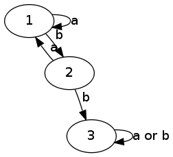
- alphabet \(\Sigma = \{a, b\}\)
- set of states \(Q = \{1, 2, 3\}\)
- transition function \(\gamma:Qc\Sigma \rightarrow Q\)
- start state \(q_o \in Q\)
- accept statues \(F \subset Q = \{1, 2\}\)
- language \(L \subset \Sigma^{*}\)
- language "recognized" by M is the set of words it accepts (e.g. no consecutive b's)
a language L is regular if there is a DFA that recognizes it
what would be an FSA which accepts any string where the 3rd to last symbol is a
machinery for proving things about FSA
- fix a language L
- for two words \(u,v \in \Sigma^{}\) - say that \(u \sim v\) if \(\forall x \in \Sigma^{}\), \(uw \in L \Leftrightarrow vw \in L\)
to prove that a language is not regular it is sufficient to provide an infinite set of mutually in-equivalent words
punchline for today – a language is regular if it has a finite number of equivalence classes under this \(\sim\) relation
2010-01-28 Thu
say that \(u \sim v\) if \(\forall w : uw \in L \Leftrightarrow vw \in L\)
the converse would be
\(u \nsim v\) if \(\exists w : uw \in L \wedge vw \notin L\)Using this \(\sim\) relation we can divide the language into equivalency classes. In the smallest possible FSA there is a one-to-one and onto correspondence between these classes and the equivalency classes.
L is regular \(\Leftrightarrow\) $∼L$ has a finite number of equivalence classes
if M and M' are both minimal machines for L, then \(M \cong M'\)
this is the Myhill-Nerode Theorem
intersections of regular languages
if L1 and L2 are regular then is \(L_1 \cap L_2\) regular? yes
The size of \(L_1 \cap L_2\) is the product of the size of their respective sizes.
once you know that the compliment of regular languages are regular, and the intersection of regular languages are regular, then you know that the compliment of the intersection of the compliments of the regular languages (which is the union : Demorgan's law) is regular
concatenation of regular languages is not as straightforward
non-deterministic finite automata (NFA)
all that matters is that \(\exists\) an accepting path
is the set of languages recognized by NFAs bigger than the set of languages recognized by DFAs. The answer is that given any DFA \(\exists\) a DFA which expresses the same thing.
2010-02-02 Tue
two points from the homework
-
when things are too obvious they can be hard to prove
(e.g. Euclid's algorithm).
Inductive proofs and structurally identical to recursive algorithms, exploit this and convert the recursive
Euclidalgorithm to an inductive proof of its validity for solving GCD.primes a = [x | x <- facts a, prime x] where facts a = [x | x <- [1..(a - 1)], a `mod` x == 0] prime a = facts a == [1]
-
in the questions about regular languages the alphabet of pairs of
bits can be combined to words which express two binary integers.
$$\binom{1}{0} \binom{0}{1} \binom{1}{1} = \binom{x}{y}$$
NFA and DFA
NFA: non deterministic finite state automata
consists of:
- \(\Sigma\) alphabet
- $Q$ finite set of states
- \(q_0 \in Q\) start state
- \(F \subset Q\) accepting states
- \(\delta : Q x F \rightarrow P(Q)\) transition function
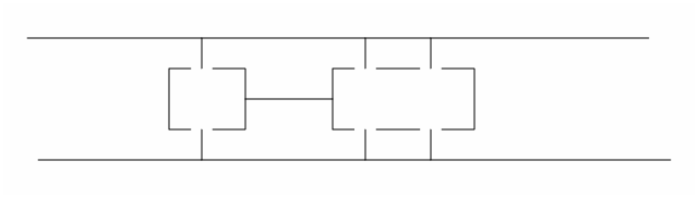
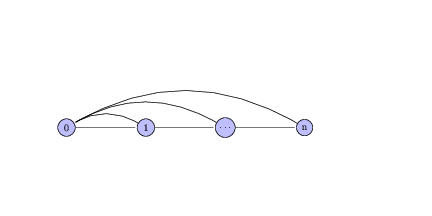
Lets apply this to another of our familiar NFAs – the language over \(\Sigma = \{0, 1\}\) where the third-to-last symbol was a 1. data/fsa.pdf
in this NFA we guess at some point that we're on the third to last symbol in the word and jump to state $b$. Note that in the above there is no legal transition out of state $d$.
lets prove that every NFA can be converted to a DFA
In effect our DFA would need to track the set of all states that we could be in were we using our NFA, and if any of those states accept.
So to define our new DFA in terms of the elements from our old NFA we get the following
- \(Q' = P(Q)\)
- \(q_o' = \{Q_0\}\)
- \(F' = \{S : S \cap F \neq \emptyset \}\)
- \(\delta'(S,a) = \cup_{q \in s}{\delta(q,a)}\)
note that \(|Q'| = 2^m\) when \(|Q| = m\) (problem 10 on hw1)
recall our language of concatenated words \(L_1L_2 = \{w : w = w_1w_2, w_1 \in L_1, w_2 \in L_2\}\) notice that while the statement "if $L$ is reg., so is \(\bar{L}\)" is obvious in the world of DFAs it is not in the language of NFAs.
regular expressions
regular expressions over the alphabet \(\Sigma\)
- \(\emptyset\) the empty set
- \(\epsilon\) the empty word
- $a$ s.t. \(a \in \Sigma\)
-
if \(\phi\) and \(\phi'\) are regular expressions then
- \(\phi + \phi'\) their concatenation is also a regexp
- \((\phi)^*\) is the continued application of \(\phi\) is also a regexp
the languages recognized by regular expressions are equivalent to the languages recognized by DFAs and NFAs etc…
partial proof by induction
-
base cases – can be recognized by DFAs
- \(\emptyset\)
- \(\{\epsilon\}\)
- \(\{a\}\)
-
inductive step
- if \(\phi\) and \(\phi'\) can be recognized by DFAs then so can \(\phi + \phi'\)
- if \(\phi\) can be recognized by DFAs then so can \(\phi^*\), for this its more convenient to use NFAs – we just wire an \(\epsilon\) transition from each accepting state back to the initial state.
2010-02-04 Thu
pumping lemma
a method of proving that a language $L$ is not regular
if L is regular, then: ∃ an integer p s.t. ∀ strings s ∈ L with |s| ≥ p ∃ strings x,y,z s.t. s = xyz, and |y| ≥ 0, |xy| ≤ p and ∀ integers i ≥ 0, xyiz ∈ L.
- basically you can pump-up the inner part of the word and continually produce words in the language
- this corresponds to loops in the FSA defining the language
- $p$ is the minimum number of steps required before you are retracing previously visited states
- note the above only has to hold for strings where \(|s| \geq p\) and there is no requirement that there need by any such strings in the language
- in languages with large words the existence of a loop in the FSA is guaranteed because the FSA must have finitely many states and once \(p \geq |FSA|\) you're set
this can be used to prove languages are not regular through contra-positive
application of the pumping lemma
negation of the pumping lemma, just flip all of the quantifiers…
using the pumping lemma to prove that the language consisting of an equal number of a's and b's is not regular.
\(\forall p\) just select the word of length \(2p\) composed of p a'sfollowed by p b's. Then it is not possible to select a sub-string in the first p letters which can be repeated – because the first p letters are all a's.
an important take home point is that we have nothing corresponding to the pumping lemma for which problems are in P (solvable in polynomial time). We don't have anything that we know must be true \(\forall\) problems in P.
context free grammars
an example: consider the following rules
- \(S \rightarrow aSb, \epsilon\) which describes the language of words with a number of a's followed by that same number of b's.
- \(S \rightarrow x,y,(S + S), (S * S)\) which results in all grammatically correct algebraic statements with paren's +'s and *'s
these context free grammars can be used to describe the programming languages which we use
This comes form linguists associated with Noam Chomsky, who believed that rules like this were how humans thought and manipulated language
regular languages are to FSAs as these grammars are to FSAs augmented with simple stacks
these grammars are context free because the left side of every \(\rightarrow\) is always a single symbol (no context) types make programs not true context free languages
where are linguists now? how does our brain really process/generate language
2010-02-09 Tue
office hours question – FSA
how to tell if an automata is the smallest possible?
there are well known algorithms for minimizing an existing DFA -- either saying yes/no this is/isn't the smallest possible, or suggesting states to merge.
two states q and q' are equivalent q ∼ q' iff ∀ w: δ*(q, w) ∈ F ⇔ δ*(q',w) ∈ F
It turns out that finding the minimal NFA is much harder because the notion of state equivalence is more complicated on an NFA.
and thus ends FSA
P, NP, and NP-completeness
NP problems are equivalent to finding a needle in a haystack – what is it about some problems that allow you to skip the exhaustive search (i.e. why can some of these problems be solved in polynomial time)?
We will repeat some material from cs561 as we discuss why some algorithms can be pulled down from NP into P.
Towers of Hanoi
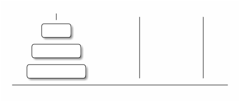
;; k is the other peg
(defn hanoi [n i j]
  (when (not (= n 0))
    (hanoi (- n 1) i k)
    (move i j)
    (hanoi (- n 1) i k)))
How many moves does it take to move n disks? \(f(n) = 2f(n-1)+1\) or \(f(n) = 2^n-1\) This can be proved optimal through induction on the number of disks.
Look at the figure in page 85 of the text to see some of the state space of this problem represented as a graph in which vertices are states and edges are moves.
If we think similarly about our computer as a large graph in which nodes are memory states and edges are moves, then the amount of memory needed is the log of the number of vertices and the runtime is the length of a path.
The optimal Towers of Hanoi algorithm is not known for more than 3 pegs.
mergesort
the canonical divide and conquer algorithm
(defn mergesort (l)
  (when l
    (let [merge ;; our sorting zipper
          lefthalf ;; left half of list
          righthalf ;; right half of list
          ]
      (merge ;; n-1 comparisons
       (mergesort (lefthalf l)) ;; f(n/2) comparisons
       (mergesort (righthalf l)) ;; f(n/2) comparisons
       ))))
What's the runtime of mergesort? Lets just count the number of comparisons.
$$f(n) = 2f(\frac{n}{2})+n$$the solution ends up being
$$f(n) = nlog_2{n}$$quicksort
(defn quicksort (l)
  (when l
    (let [pivot ;; choose our pivot
          lp    ;; elements less than p
          gp    ;; elements greater than p
          ]
      (concat (quicksort lp) p (quicksort gp)))))
- n comparisons to get greater and less than pivot
- if our pivot is really in the middle then we have \(2f(\frac{n}{2})+n\) more comparisons
- if our pivot is the smallest element, then we have \(f(n-1)+n\) comparisons which becomes the arithmetic series \(1 + 2 + 3 + \ldots\) which is \(\Theta(n^2)\)
-
in the average case where p is randomly placed in our list and $a$
is the fractional amount of p through our list, then we have
\(f(an)+f((1-a)n)+n\) – then setting \(f(n)\) as the average over all
possible values of $a$.
$$f(n) = (n - 1) + \frac{1}{n} \sum_{i=0}^{n-1}{f(i) + f(n - 1 - i)}$$
when $n$ is large we can replace this sum by an integral
$$f(n) = n + \frac{1}{n} \int_{0}^{n}{d_x f(x) + f(n - x)}$$
we can try to substitute in \(f(n) = An\ln{n}\) and solve for $A$
this is our first example of a randomized algorithm
be sure to be explicit about what your input could be
- designed by an adversary
- truly random
- real world
2010-02-11 Thu
sorting runtimes
Can we sort n things in less than \(n\log_2{n}\) comparisons
To distinguish N possibilities with binary (yes/no) questions you will need to ask \(\log_2{n}\) questions.
when there are n! sortings of a list, to select the correct one will require \(\log_2{n!}\) questions
$$\log_2{n!} = n\log_2{n} - n\log_2{e} - O(\log_2{n})$$or \(O(n\log_2{n})\)
note: this argument is based upon the minimum amount of time taken for our sorting algorithm to access the information in the list – not the trivial computation performed on the list info after it is known to the algorithm.
radix-sort and bin-sort are faster non-comparison based sorting algorithms that are applicable in some cases.
modular exponentiation and discrete log
-
mod. exponentiation
- input
- n-digit integers x, y, p
- output
- \(x^y \bmod{p}\)
- discussion
-
if \(y=1024\) then since \(1024 = 2^{10}\) we can just
do \(x = x^2 \bmod{p}\) 10 times
for values of y which are not power of 2 we can just run out powers of 2 trick up to the nearest power of below y, this is another divide and conquer algorithm
this runs in poly time and is in P
if we have time at the end of the semester we'll look at some cryptography stuff which will relate here.
-
discrete log
- input
- n-digit integers x, z, p
- output
- y s.t. \(z = x^y \bmod{p}\)
- discussion
- this function doesn't appear to be in P even though its inverse above is in P
These functions in which one direction is in P while the inverse isn't are called one-way functions. There are some cool one-way functions, like generating random sequences which are so random that no poly-time algorithm can find a pattern in them.
fast Fourier transforms
are very important for many day-to-day applications, and are vital to understanding quantum computing and its ability to crack RSA keys, etc…
dynamic programming
For example putting line breaks into a paragraph.
need to assign some cost to each line based on how stretched its words are. namely the total space in the line - the amount of space taken by the words.
$$c(i,j) = (line\_space - \sum_{k = i}^j{length(w_k)} - (i-j))$$So taking a divide-and-conquer approach, we continually place a line break into the paragraph dividing the paragraph into two sub-paragraphs which we can then typeset. However it is not at all clear a-priori where the best initial divisions will be.
taking a dynamic programming approach we will place a line break after the first line and assign that break the cost of that line break as the cost of that line, plus the cost of the remained of the paragraph type-set as well as possible.
side note: short-vs-long term costs – there is a relevant book by the guy who talked on Colbert recently
(defn typeset-cost
  "Return the lowest cost of typeseting a paragraph of WORDS as well
  as possible" [words cost]
  (min (map
        (fn [break]
          (+ (cost (take break words))
             (typeset-cost (drop break words))))
        (range (.size words)))))
this would be very inefficient because we are continually
recalculating the cost of the same paragraphs. however we can cache
our intermediate results as in the following – also since its in
clojure its multithreaded with safe access to the cache.
(def cache (ref {}))

(defn typeset-cost
  "Return the lowest cost of typeseting a paragraph of WORDS as well
  as possible -- with thread-safe caching." [words cost]
  (or (@cache words)
      ((dosync assoc @cache words
              (min (pmap
                    (fn [break]
                      (+ (cost (take break words))
                         (typeset-cost (drop break words))))
                    (range (.size words)))))
       words)))
this brings us down from an exponential runtime to a polynomial runtime.
so
- dynamic programming
- recursion with memorization
this is typically applicable to string and to trees – problems which can be cut into separate problems in a polynomial number of places.
2010-02-16 Tue
minimum spanning tree
minimum spanning tree
- input
- a weighted graph \(G = (V,E)\)
- question
- spanning tree T, smallest total weight
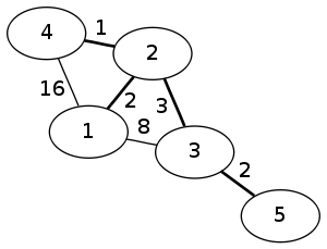
greedy algorithm: Kruskal's alg., sort E from lightest to heaviest add each one if this doesn't create a cycle.
-
proof: we will maintain the invariant, that the set of edges we
have so far, \(F \subseteq E\) is contained in some minimal spanning
tree (MST) $T$.
initialization(base case): \(F = \emptyset\)
termination: left as an exercise
maintenance(inductive step): if \(F \subseteq T\) s.t. $T$ is a MST then \(F \cup \{e\} \subseteq T\). Proof by contradiction, suppose that \(e \notin T\), then \(\{e\} \cup T\) has a cycle which means that any of the edges in that cycle could be removed and you would still have a minimum spanning tree, since $e$ was the smallest remaining edge one of the other edges has a greater or equal weight than $e$, \(\square\).
Note that for the traveling salesman problem (a simple restriction of this problem) a greedy algorithm performs very poorly.
max flow
max flow
- input
- directed graph with two special verticies, the source (s) and the sink (t), and each edge has a capacity
- question
- what is the maximum flow from s to t in the graph
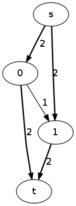
improvement algorithm: if I have a flow $f$ (a path from s to t), I can tell if $f$ is optimal and if it isn't then I can tell how to improve it.
all of the parts of this algorithm will be polynomial in the size of the graph – including the bits needed to encode the capacities of the edges.
proof: $f$ is optimal unless \(\exists\) a path $p$ from s to t s.t. \(\forall e \in p\), $e$ has nonzero residual capacity – not quite true
residual graph: given a current flow $f$, the graph \(G_f\) has forward edges e with capacity \(c_f(e) = c(e) - f(e)\), and reverse edges \(\bar{e}\) with capacity \(c_f(\bar{e}) = f(e)\) amended proof: $f$ is optimal unless \(\exists\) a path $p$ in the residual graph, from s to t s.t. \(\forall e \in p\), $e$ has nonzero residual capacity. flow along a reverse edge cancels out flow along the related forward edge.
Refer to the book for the proof.
note that the number of iterations through this, path -> flow -> residual -> path loop is run could be infinite w/real-number capacities, and can take an exponential number of trials if the capacitances are exponentially large.
note in a fitness landscape, local optima only exist if there is an idea of small changes, so broadening the set of small changes can remove local optima and smooth a fitness landscape
reduction/transformation between problems
min cut
- input
- given a weighted graph
- question
- find the cut \(C \subseteq E\) which eliminates all paths between s and t and minimizes the capacity of the edges cut
in every case the weight of the minimum cut is equal to the maximum flow – intuitively this should be clear, each problem find the bottleneck between two subgraphs containing s and t.
a reduction from problem a to problem b is a poly-time translation of instances of a to instances of b.
here's one more example of a problem amenable to reduction/translation
Bipartite perfect matching
- input
- bipartite graph $G$
- question
- find a set of edges s.t. every vertex is contained in exactly one edge.
this is reducible to max flow, through adding s to one bipartite half, and adding t to the other bipartite graph, and ask if there is a flow of value n – every edge along compatibility graph is given a flow of 1.
so, Perfect Matching \(\leq\) Max Flow
2010-02-18 Thu
un-skipping part of section three – Reachability
Reachability
- input
- directed graph G and two verticies s, t
- question
- is there a path from s -> t
it is common to ask for the shortest path (either weighted or not)
-
middle first search – as opposed to breadth first or depth first
we will be using an adjacency matrix
\begin{displaymath} A_{ij} = \left\{ \begin{array}{lr} 1 & : (i,j) \in E\\ 0 & : (i,j) \notin E \end{array} \right. \end{displaymath}
Raising A to powers gives us \(A^n_{ij} = \sum_k{A_{ik}A_{kj}}\) gives us the number of paths of length $n$ from $i$ to $j$.
we can quickly get to high powers of \(A_{ij}\) using modular-exponentiation
how would this look at code
(defn reachable?
  [A s t]
  (loop [A A
         n 0]
    (if (A s t)
      (if (>= n (.size A))
        nil
        (recur (matrix-square A) (inc n))))))
if you're looking for the shortest path your initialization may want to look something like
\begin{displaymath} A_{ij} = \left\{ \begin{array}{ll} 0 & i \equiv j\\ 1 & (i,j) \in E\\ \infty & (i,j) \notin E \end{array} \right. \end{displaymath} would solve the all pairs shortest path problem
on to Chapter 4 – NP
decision problems (yes/no)
- p
- polynomial time problems – ∃ a program running in poly(n) time which solves the problem where n is the size of the input measured in bits
- NP
- class of problems where checking a solution is in P – the class of problems where the answer is "yes" if ∃ w : B(x,w) where B ∈ P (we call w the witness)
- coNP
- the class of problems who's compliment is in NP, for example proving that a graph does not have a Hamiltonian path
a tour of problems in NP
Graph k-colorability
- input
- graph
- question
- is there a coloring of the vertices using k colors s.t. no two vertices of the same color share an edge
this is in NP as the witness can be checked in poly time
we think this takes exponential time
the 4-colorability of planar graphs was proved with a computer-aided search in the 1970s
Graph 3-colorability \(\subseteq\) planar graph 3-colorability -- through the introduction of little gadget graphs at each intersection
2010-02-23 Tue
some points related to the homework
-
problem 2
the point of problem 2 was a language which is not regular, but which does satisfy the pumping lemma.
closure properties means taking the languages union, intersection, or compliment or any of those actions which preserve regularity, and then show that the resulting languages is not regular.
-
factoring
- input
- n-bit integer x
- output
- a list of prime factors \(p_i\) and integers \(t_i\) s.t. \(x = \prod_{p_i}{t_i}\)
see the hint on the list – note that factoring can be reduced to the find a factor problem.
so the easiest setup is FACTORING \(\leq\) FIND A FACTOR \(\leq\) MOD. FACTORIAL
- there is also the divide and conquer problem with Fibonacci numbers – not that if the given recursion is used directly the result is poly(l), but maybe not in the number of bits in l – it needs to be polynomial in the number of bits in l \(poly(n=log_2{l})\)
-
finally some terminology related to dynamic programming, shared subproblems – means basically exactly what the name sounds like --
its related to the Hamiltonian path problem
naively this would be checking the n! vertex orders where \(n! \sim n^n \sim n^{O(nlog{n})}\)
more Chapt. 4 – problems in NP
- k colorability
NP, ∀ yes instances ∃ a witness, example, or certificate of the solution which can be checked in poly timeGraph k-coloring
- input
- G
- output
- is G k-colorable
last time we mentioned the surprising fact that graph 3-coloring \(\leq\) planar graph 3-coloring
- satisfiability
CNF (in terms), any formula/truth-table can be represented in CNFa truth assignment is an assignment of each variable to either true or false.
φ is satisfiable if ∃ a truth assignment for which φ is true
SAT
- input
- a CNF formula φ
- output
- is φ satisfiable
this is clearly in NP, its easy to check a truth assignment. proving unsatisfiable is pretty hard
KSAT
- input
- a CNF formula φ with k literals in each clause
- output
- is φ satisfiable
graph 3-coloring \(\leq\) SAT
- one variable for each vertex and color combination
- one clause for each edge and color combination
- four clauses for each variable
once you get used to this you realize that its easy to convert most constraint satisfaction problems into a SAT problem – and this is something that is actually done in the real world where smart people spend real time working on efficient sat solvers.
2010-02-25 Thu
2 and 3, and SAT -> graph
-
coloring
- 2-coloring is in P
- 3-coloring isn't in P
-
SAT
- 2-SAT is in P
- 3-SAT isn't in P and is equivalent to every other k-SAT
p. 112
\(\phi(p,q,r) = (p \vee \bar{q}) \wedge (\bar{p} \vee \bar{r}) \wedge (q \vee r) \wedge (p \vee q)\)

the formula is satisfiable iff \(\nexists\) a cycle including both $x$ and \(\bar{x}\) for some $x$.
while there are unset vars…
- choose unset x
- if path x -> \(\bar{x}\), set x false
- if path \(\bar{x}\) -> x, set x true
- else set x however you want
then do unit clause propagation
note that edges in this graph come in pairs, so x -> y means \(\bar{y}\) -> \(\bar{x}\)
its tempting to do something similar for 3-SAT, however we can't
k-SAT <= 3-SAT
Thus far we've only done gadget reductions, where we make simple substitutions to get from one problem to another, however for problem reduction we can do anything which can be accomplished in polynomial time
reduction of a 5-variable clause to a 3-variable clause
$$(x_1 \vee x_2 \vee x_3 \vee x_4 \vee x_5)$$goes to
$$(x_1 \vee x_2 \vee z_1) \wedge (\bar{z_1} \vee x_3 \vee z_2) \wedge (\bar{z_2} \vee x_4 \vee x_5)$$what's qualitatively different between 2 and 3
NP-completeness – enough beating around the bush, Chapt. 5
a problem A is NP-complete if
- A ∈ NP
- ∀ B ∈ NP, B \(\leq\) A (there is a poly-time reduction from B to A)
-
Prove 3-SAT is NP complete
if B is in NP, then ∃ a program C(x,w) that returns true iff w is a valid witness for x, where x is a yes-instance of B.
lets replace the word program above with circuit. so we compile our program all the way down to Boolean circuits converting the input bits to outputs bits.
claim: given an instance x of B, we can generate a circuit c'(w) s.t. c'(w)=true iff w is a valid witness for x. this is a reduction form B to CIRCUIT-SAT
CIRCUIT-SAT
- input
- a boolean circuit c'
- output
- is there an input x s.t. c'(w) = true
so we've shown CIRCUIT-SAT is NP-complete
reduction is transitive, so if CIRCUIT-SAT \(\leq\) 3-SAT then 3-SAT is also NP-complete
WITNESS EXISTENCE \(\leq\) CIRCUIT-SAT \(\leq\) 3-SAT
we can take an instance of circuit-sat, assign variables to all internal wires, we can then in a fairly straightforward manner turn a circuit into a k-SAT problem which ends in \(\wedge (z)\) where $z$ is the variable for our output. So how do we know this is poly-size of the original circuit, seems like it may be obvious, possibly only one clause per-wire.
Summary: any program, take its witness-checker to a circuit, convert that circuit to a 3-SAT formula, that formula is satisfiable iff a witness exists.
2010-03-02 Tue
NAE-k-SAT
NAE-k-SAT – not all equal satisfiability
- input
- a finite conjunction of clauses of k variables
- output
- is there an assignment of variables s.t. each clause contains at least one literal that is true and one that is false
note that true and false are totally equivalent in this specification, so for any solution, swapping true and false will yield another solution
NAE-2-SAT ∈ P
NAE-2-SAT \(\leq\) Graph 2-coloring
just say that every literal is a vertex, every literal is connected by an edge to its compliment, and every clause is an edge
3-SAT <= NAE-SAT
3-SAT \(\leq\) NAE-4-SAT \(\leq\) NAE-3-SAT
so this \(leq\) relation in NP problem reductions requires that we can map no and yes instances between the two problems – in this case 3-SAT and NAE-4-SAT
- to convert form 3-SAT to NAE-4-SAT
$$(x_1 \vee y_1 \vee z_1) \wedge (x_2 \vee y_2 \vee z_2)$$becomes
$$(x_1, y_1, z_1, b) \wedge (x_2, y_2, z_2, b)$$where $b$ is added to every clause, and can be set to either true or false
so, the intuition here is that if 3-SAT is not satisfiable, then there must be one clause of all false, and one clause of all true, because if that is not the case, then we can just swap our true and false assignments, and then if there is a clause of all false, and there is not a clause of all true, then the swapped values will satisfy. So the above is not NAE-4-SAT iff there is a clause of all true and one of all false.
- now to show that NAE-4-SAT \(\leq\) NAE-3-SAT
we add variables to reduce the size of clauses
$$(x_1 \vee y_1 \vee z_1 \vee t_1)$$becomes, just need to know what new variables are inserted
$$(x_1 \vee y_1 \vee \_) \wedge (x_1 \vee z_1 \vee \_) \wedge \ldots$$
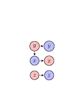
3-SAT <= 3-coloring
another gadget reduction, here generating graphical representations of clauses
types of gadgets
- choice
- where you set the values to one of the possible values
- constraint
- where you force two or more variables to obey a constraint
so we can make one color true, one false, and then the other can be used to enforce constraints, so for example
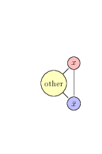
with this gadget forcing each variable and its compliment to be different colors, how do we convert our clauses into subgraphs of our graph.
turns out we'll use NAE-3-SAT to generate these subgraphs, then the subgraphs just turn into fully connected graphs of three vertices, or triangles, that way they will not be three colorable if all three vertices outside the subgraph with incoming edges are the same color – or NAE.
2010-03-04 Thu
reduction of sorting to graphs, consider a graph where each vertex is a number, and we draw directed edges between vertices from the smaller to the greater (representing the less than relation)
then sorting can be reduced to a Hamiltonian path through this graph
this was to make a point about the directions of reductions, sorting is not as hard as Hamiltonian paths
sidebar – DAGs and topological orderings
if a DAG is a partial ordering, then the topological orderings related to that DAG are all of the possible total orderings which do not violate the partial ordering of the DAG.
back to SAT
- clause
- is a disjunction of terms
- assignment
- is a grounding of the literals in a collection of clause causing their conjunction to be true
since we know 3-SAT is NP-Hard we'll use it to prove that other problems are NP-Hard
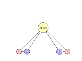
independent set is NP-Hard
INDEPENDENT SET
- input
- a graph G
- question
- is there a set of vertices which share no edges
- in NP
- this is trivially in NP, because we can check any set of vertices in polynomial time
- in NP-Hard
- can we reduce 3-SAT to independent set, for each clause introduce a connected subgraph (triangle) where the vertices are the variables in the clause. Then connect each vertex to each of its opposites, so $x$ is connected to every \(\bar{x}\), then finding a independent set with size equal to the number of clauses will result in a satisfying vertex assignment for 3-SAT.
clique is also NP-Hard
CLIQUE
- input
- a graph G
- question
- is the a collected subgraph of size k
this is exactly the same as independent set of the compliment of the graph
vertex cover
VERTEX COVER
- input
- a graph G
- output
- set of vertices of size k s.t. every edge in G touches one of those vertices
If you have a clique of size k in the compliment graph of G, then you have a vertex cover of size |V|-k in G.
proof – if there was an edge not covered by the non-clique in the compliment of G, then that edge would mean that the clique in compliment of G was not fully connected.
set cover
SET COVER
- input
- given a set A on n elements and a family F of subsets of A
- question
- is there a sub-family of F whose union is A
trivial
2010-03-09 Tue
NP-COMPLETE review
WITNESS-EXISTENCE
- input
- an instance and a program that checks witnesses to the instance
- question
- is there a witness that satisfies this instance/program
- ???
- we can compile this to an instance of CIRCUIT-SAT
- ???
- which we can convert to a 3-SAT problem
- ???
- which we can convert to a NAE-3-SAT problem (through NAE-4-SAT)
- ???
- which we can convert to GRAPH-3-COLORING
- 3-SAT to NAE-3-SAT
looking once more at the 3-SAT to NAE-3-SAT (through NAE-4-SAT)- we can take any 3-SAT instance and add a variable $S$ to each clause generating an instance of NAE-4-SAT
- and some more… just be sure that you can map yes instance to yes instances, and no instances to no instance
- NAE-3-SAT to GRAPH-3-COlORING
Now for some problems with a different flavor
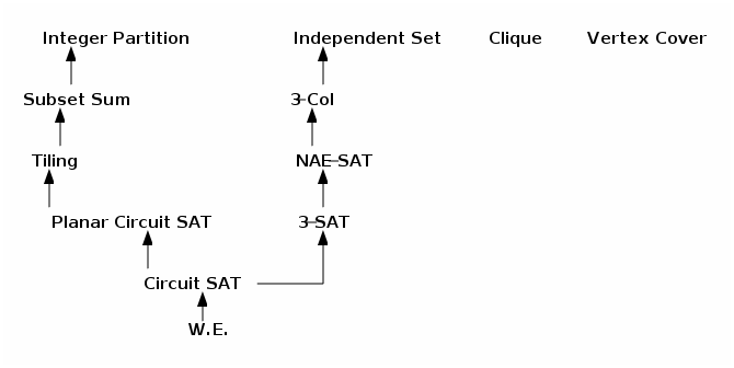
TILING
- input
- set of rotatable tile shapes T, and a finite region R
- question
- can I tile R with tiles from T w/o gaps or overlaps
for simplicity we'll say both the tile shapes and the region are made of unit squares, and they will be conveyed as gif images (basically images of bits)
our tile set will be little elbows and squares
|    +--+
+--  |  | :      +--+
we can use these shapes to make wires and gates (see the book) s.t. truth values are based on the how the little elbows are aligned in the wires…
the last output can be setup so that its only covered if the wire heading to it is aligned as true, so the whole shape is tilable iff the analogous circuit would have returned true.
so tiling with these shapes is NP-Complete
tiling with dominoes is in P
- convert R to a bipartite graph by coloring the vertices as a checker board
- then domino covering is equivalent to bipartite perfect matching, which is equivalent to max flow
some weird relationships between improving imperfect domino matching and the Ford-Fulkerson algorithm for improving max flow
once again the difference between 2 and 3 is made manifest, if someone really understood this basic difference that insight should lead to a proof that \(P \neq NP\).
Integer Partition
introduced in section 4.2.3
INTEGER PARTITIONING
- input
- a list of integers {x1,… , xl}, note: n is the number of bits, so its possible for xl >> n
- question
- is there a balanced partition of this list of integers? \(A \subseteq \{1, \ldots, l\}\) s.t. \(\sum_{i \in A}{x_i} = \frac{1}{2}\sum_i{x_i}\)
this is a special case of SUBSET SUM in which we want the sum of elements in $A$ to equal some sum $t$ – this is in NP
we can try this with dynamic programming…
2010-03-23 Tue
review of the reduction tree
Cosine Integrals
NP-Complete problem from calculus
COSINE INTEGRALS
- input
- list of integers a1, a2,…, an
- question
- is $$\int^{\pi}_{\pi}{d\theta (\cos{a_1 \theta})(\cos{a_2 \theta})\ldots(\cos{a_n \theta})} \neq 0$$
this is actually integer partitioning in disguise
- recall $$cos\theta = \frac{e^{i\theta} + e^{-i\theta}}{2}$$
- then we have \begin{eqnarray*} \prod^n_{j=1}{\cos{a_j \theta}} &=& \frac{1}{2^n}\prod^n_j{e^{ia_j\theta} + e^{-ia_j\theta}}\\ &=& \frac{1}{2^n} \sum_{A \subseteq \{1,\ldots,n\}}{\left(\prod_{j \in A}{e^{ia_j\theta}} \prod_{j \notin A}{e^{-ia_j\theta}}\right)}\\ &=& \frac{1}{2^n} \sum_{A \subseteq \{1,\ldots,n\}}{e^{i\theta} \left( \sum_{j \in A}{a_j} - \sum_{j \notin A}{a_j}\right)} \end{eqnarray*}
- which equals 0 iff A is a balanced partition
- so, in fact the entire integral is equal to $$\frac{2\pi}{2^n}(\text{\# balanced partitions})$$
so, telling whether the integral is non-zero is NP-complete, however actually computing the integral is much harder, in general the non-decision version of an NP problem is in #P (pronounced count P)
primality is in NP
if p is a prime, then the set of non-zero integers mod(p), or the set {1,…,p-1} form a group under x
a group requires an operator . which is
- closed in the group
- associative meaning a.(b.c)=(a.b).c
- has an identity element e, s.t. a.e=e.a=a
- has inverses, ∀ a ∃ a-1 s.t. a.a-1=a-1.a=e
- (abelian groups also have this property) a.b=b.a
p has to be prime to ensure the existence of multiplicative inverses. generally every element that is mutually prime with n has an inverse mod(n).
a cyclic group is a group generated by a single element a: $$\{1, a, a^2, \ldots, a^r=1\}$$ if p is prime, \(\mathbb{Z}^*_p\) is cyclic. the generator = "primitive root"
example
- p = 5
- a = 2 is a primitive root because its powers generate everything in the group with the powers, {1, 2, 4, 3, 1, 2…}
Theorem: p is prime, iff ∃ a primitive root a.
a is primitive implies,
- $$a^{p-1} \equiv_p 1$$
- $$\nexists t | 0<t<p-1 s.t. a^t \equiv_p 1$$
this is all to show that using a as our witness we can show p is prime in poly-time
- easy to check $$a^{p-1} \equiv_p 1$$, because modular exponentiation is in P
-
checking all of the values of t
- we only have to check values of t which divide p-1
- however an n-bit number can have more than a polynomial number of divisors
- so we claim: if ∃ t<p-1 s.t. $$a^t \equiv_p 1$$, then ∃ a prime q which divides p-1, s.t. $$a^{\frac{(p-1)}{q}} \equiv_p 1$$
- luckily the prover who gave us our witness will need to give us both the primitive root a, and the prime factors of p-1, the combination of which is called Pratt's primality certificate for p
-
Pratt's primality certificate for p
- a primitive root a
- prime factorization of p-1, \(p-1=q^{t_1}_1q^{t_2}_2\ldots q^{t_l}_l\)
- as well as Pratt certificates for q1, q2, etc…
so we just make sure that the total size of all these Pratt certificates is poly-size
- the total number of bits in q1…ql is at most n
- each time we recurse things get significantly smaller, and we'll only recurse down n levels
- so n levels of n bits = O(n2)
primality *is* in NP
- 70s – primality is in NP
- 60s – randomized algorithms for finding primes in poly time
- 04 – deterministic algorithm in something like n12 time
2010-03-25 Thu
next two chapters are both fun/philosophical – conceptual depth with technical ease
Note: definitely read section 6.1.3
why is P vs. NP so hard?
Seems intuitively obvious, but seems very hard to prove.
The Clay Mathematics Institute poses 7 questions including the great remaining unsolved problems in mathematics, including this problem.
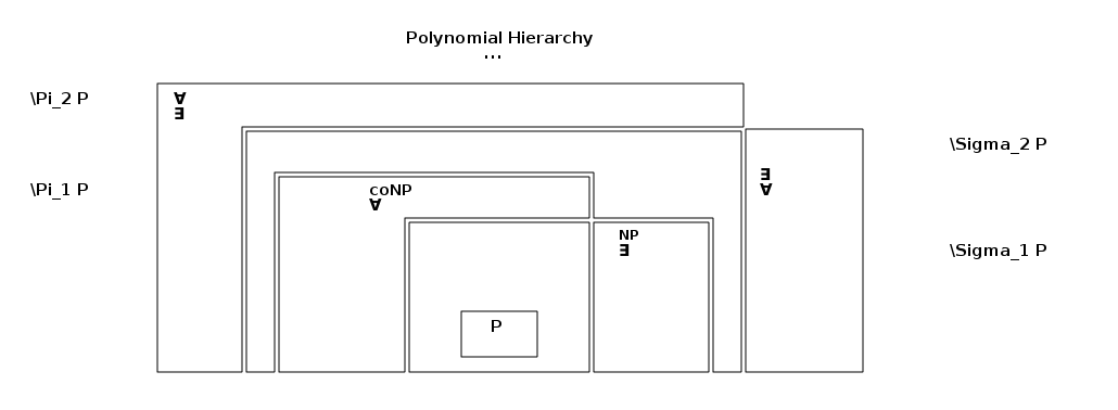
what if P+NP
polynomial hierarchy – $$PH = \cup^{\infty}_{i=1}{(\sum_i{P \cup \prod_i{P}})}$$
SMALLEST BOOLEAN CIRCUIT
- input
- a Boolean circuit C
- question
- is C the smallest possible circuit that computes fc?
how many quantifiers would this problem require?
- \(\exists c'<c: \forall w: f_{c'}(w) = f_c(w)\)
- \(\forall c'<c: \exists w: f_{c'}(w) \neq f_c(w)\)
- in fact the circuit difference sub-problem is in NP
the building of ∀ and ∃ quantifiers is similar to claiming a winning strategy in chess, you need to be able to say that
- ∀ moves by your opponent ∃ a move by you s.t. some poly-time property is still true
- or ∀ opponent moves, ∃ a move s.t., ∀ opponent moves, ∃ a move s.t. etc…
if P=NP then the entire polynomial hierarchy collapses into P
because P is closed under compliment, NP=P -> coNP=P=NP, meaning you could just start absorbing ∃ and ∀ quantifiers and everything else would also end up in P
P-space
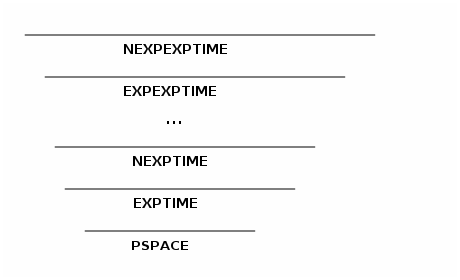
if P=NP then TIME(f(n))=NTIME(f(n))
- proof
-
suppose A ∈ NEXPTIME, input is n bits long and a witness can
be checked in time \(t(n)=2^{O(n^c)}\).
pad out the input: add t(n)-n 0's, now it has length \(n'=t(n)\) bits, and the witness can now be checked in time \(t(n)=n'\).
this new padded problem is then in NP, but if P=NP then its in P, which means it can be solved in poly(n') time, however \(poly(t(n))=2^{O(n^c)}\) which means that A ∈ EXPTIME
cryptography
P=NP -> modern cryptography does not work
encryption in polynomial time -> decryption is in NP
theorem proof
PROOF CHECKING
- input
- set of axioms A, statement S, proof P (collection of axiomatic statements)
- question
- is P a valid proof of the statement S
SHORT PROOF
- input
- axioms A, statement S, integer L (in unary, to make things easier)
- question
- is there a valid proof P of S which is < L statements long
so, if P=NP then we can tell if proofs exist at arbitrary length in poly(length) time.
Goedel's question to Von-Neuman
let φ(n) = time it takes for the optimal machine to search for proofs up to length n.
then the mental effort of mathematicians in resolution of yes/no questions could be replaced by machine.
he had a note in margin that mathematicians could still be creative in creating axioms
2010-03-30 Tue
introduction to time hierarchies
It is surprising how few ways we have for proving lower bounds on the runtime of an algorithm.
one of these is diagonalization.
we will construct some artificial problems which can be solved in \(n^{2.0000001}\) time, but can not be solved in \(n^{2}\) time. PREDICTION
- input
- a program Π and an input x
- question
- if Π(x) halts within f(|x|) steps, return Π(x) (the output), however if Π(x) takes > f(|x|) steps then return "don't know"
is there a faster way to get the output of a program, then running the program itself.
in the above "f(|X|)" is the running time of the complexity class you want to "get out of". in that case PREDICTION is outside of the class of problems which can be solved in exactly f(|n|) steps or TIME(f(n)), but it is inside of a larger class TIME(g(n)). by this the existence of PREDICTION proves that ∃ g(n) and that \(f(n) \subset g(n)\)
diagonalization
CATCH22
- input
- a program Π which returns yes/no answers
- question
- suppose Π is given its own source code as input, Π(Π). if it halts within f(|Π|) steps, then return the opposite of Π(Π), else return "don't know"
notice that CATCH22 is a special case of prediction
feeding CATCH22 to itself is a contradiction, so it takes more time than previously.
time hierarchy theorem
If our programming language model of computation lets us simulate t steps of an arbitrary program Π, while running a clock that goes off after t steps in S(t) time, and if g(n)=o(f(n)), then \(TIME(g(n)) \subset TIME(S(f(n)))\)
why can't we prove P ⊂ NP w/diagonalization
this could happen in PREDICT were in NP
its not in NP because to check programs running in higher and higher poly times, there is no fixed poly time which can check all fixed poly times, sort of like how the greatest \(n \in \mathbb{N}\) is \(\infty\). Relativized complexity
- PA
- class of problems we can solve in poly(n) time given access to an oracle for A. (call subroutine for A in poly time)
- NPA
- ditto only for checking in PA
∃ problems A,B s.t. PA=NPA but PB ≠ NPB
A proof technique relativizes if it works in all possible worlds, i.e. if it proves that C ≠ D, then CA \new DA
diagonalization relativizes, and no relativizing technique can prove that P ≠ NP.
Q-SAT
recall the hierarchy of NP and coNP classes differentiated by their quantifiers (∀ and ∃)
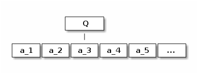
Quantified SAT
- input
- a quantified Boolean formula ∃ x1: ∀ x2 … ∃ xn : φ(x1,…xn) = Φ
- question
- is Φ true?
this problem lives in P-SPACE above our hierarchy. in fact it is P-SPACE complete meaning it is the hardest problem solvable with polynomial space an infinite time.
we claim that \(P^{Q-SAT}=NP^{QSAT}\), this is true because no matter our world, NP is just P with one more quantifier in front of it, but QSAT with another quantifier is just another instance of QSAT
haystack oracle, B
The oracle will say "yes" to at most one sn of each length n.
∀ n > 0 we flip a coin
- heads
- choose a random bit string Sn of length n and add it to S
- tails
- we don't add anything to S of length n
FINICKY ORACLE
- input
- n in unary
- question
- does B (haystack oracle) say yes to any string of length n
trivially in NPB, however not in PB because you have to guess a single random string out of 2n possible strings, so you can't reliably find the random string with a poly number of guesses
2010-04-01 Thu
review of the midterm questions (see the midterm-solutions.pdf)
we are strongly urged to convince ourselves of the following $$ \sum_{t=0}^n{\binom{n}{t}2^t} = 3^t $$ note that in problem 5, the "insert a vertex in each edge" gadget needs to be extended by completely connecting all of the inserted vertices.
start reading chapter 7 – its very fun
2010-04-06 Tue
- we will not cancel class on Thursday, it will be up on video (link will be sent to the email list, http://mts.unm.edu/Cs_courses.html)
- we should really do ourselves a favor and read Chapt. 7
a couple of tidbits from Chapt. 6
the take home point of the following is that there is some significant inner structure inside of P and NP
-
if P ≠ NP then ∃ problems which are in between, i.e. are
not in P and are not NP-Complete. a couple of problems people
believe are in between are
- factoring
- graph isomorphism – is almost always in P
-
if any problem in NP ∩ coNP is NP-complete, then NP=coNP, this
would mean that whenever you have a poly-time property P whith a
∃ P you could change it to a poly-time property with a ∀
P, or rather existence statements and non-existence statements would
be equivalent
This means that the entire polynomial hierarchy would collapse because two consecutive existential quantifiers of the same type can be collapsed, e.g. (∃ ∀) would be equal to (∃ ∃) which collapses to (∃)
-
total function NP (TFNP) – witness always exists but is hard to find
-
pidgin subset
- input: a list of integers x1 … xl
- output: a pair of subsets A ≠ B ⊂ {1, …, l} s.t. $$\sum_{i \in A}{x_i} \equiv_{2^l} \sum_{i \in B}{x_i}$$
- see Chpt. 6 for more information, but this relates to non-constructive proofs, and to a new complexity class of things that can't be found in P, but the pidgin hole principle can proof that they exist in P (PPP). if P and NP collapse, then pidgin hole proofs can be used as constructive proofs
-
pidgin subset
some early programming history
the grand unification of 1936
-
1800s
- Leibniz was the first to build machines to compute functions
- Babbage was the first to try to build a machine which could compute a wide variety of functions namely polynomials (his Differential Engine), and he wanted to be able to mechanically compute series of instructions (his Analytical Engine) (1840s), he was inspired by a type of programmable loom
- Ada Augusta, Lady Lovelace (the illegitimate daughter of Lord Byron) can be considered the first programmer as she wrote a non-trivial program for Babbage's Analytical Engine. She was also among the first to imagine the use of computers beyond simply numerical functions
-
1900s – (Hilbert, Church, Turing, Godel)
-
Hilbert was a formalist – meaning he hoped that mathematics could
be "completed", that given the right axioms and enough work every
true mathematical statement could be proven. He is responsible
for the "Decision Problem".
around this time people were trying to "formalize" math with Set Theory.
on Thursday we'll prove Godel's incompleteness theorem.
-
Hilbert was a formalist – meaning he hoped that mathematics could
be "completed", that given the right axioms and enough work every
true mathematical statement could be proven. He is responsible
for the "Decision Problem".
Recommended Reading
- logicomix is a comic book about Bertrand Russel and the foundations of mathematics.
- Godel, Escher, Bach – Hofstadter
some discussion of the different cardinalities of ∞ (see cardinality of sets – sizes of infinity in the cs550 notes)
Russel's Paradox: The set of all sets that do not contain themselves. this paradox led to a stratified structure of sets s.t. no set can refer to sets on the same or lower levels
| ∅ |
| integers |
| sets of the above |
| \(\vdots\) |
2010-04-08 Thu
- see video http://mts.unm.edu/Cs_courses.html
- ensure comfort with recursive enumerability
2010-04-13 Tue
skim section 7.4, read 7.5
a couple of words about the homework
-
for any f(n)
$$ NTIME (f(n)) \subseteq TIME(2^{O(f(n))}) $$
- yes-instance have witnesses w of size |w|=O(f(n)) which can be checked in O(f(n)) time
- there are \(2^{|w|} = s^{O(f(n))}\) possible witnesses, each of which takes O(f(n)) time to check so \(2^{O(f(n))} \times O(f(n)) = 2^{O(f(n))}\) time to check all witnesses
$$ NTIME (f(n)) \subseteq TIME(2^{O(f(n))}) \subseteq NTIME(2^{O(f(n))}) \subseteq TIME(2^{2^{O(f(n))}}) \ldots$$
-
Monier-Speckenmeyer – 3-SAT solver with better than 2n time
1.8n << 2n
clause
x1 x2 x3 <- a clause and its variable assignments T if this leads to a contradiction then try… F T if this leads to a contradiction then try… F F T is better than naively trying all possible assignments to each variable.
-
we can prove problems are undecidable by reducing the halting
problem to them
Rice's Theorem: any long-term question about the behavior of a program is undecidable
foundations
programs being both code and data, similar to DNA/RNA being both the passive information storage data and also being enzymes which are active and can modify the original DNA data like a program
main models of computation
initial explorations into programming were performed by logicians trying to build up complex functions from a primitive set of basic functions.
- primitive recursive functions :: building functions on \(\mathbb{N}\)
from the following primitive set- 0(x) = 0
- S(x) = x + 1 – note "+" is not yet defined in this language,
just used for the gist of its meaning
- I(x) = x
- \(I^3_2(x, y, z) = y\)
Some functions on functions
- composition. \((f \circ g)(x) = f(g(x))\)
- primitive recursion. if f(x), g(x,y,z)
- base case h(x,0) = f(x)
- recursive step h(x,y+1) = g(x,y,h(x,y)) – not that by
definition the value of the recursive variable "y" must decrease with every nesting of recursion.
- examples with simple arithmetic
- addition
(defun add (x y)
(if (= x 0) x (successor (add x (predecessor y)))))
- multiplication
(defun mult (x y)
(if (= x 1) x (add x (mult x (predecessor y)))))
- by definition there is no primitive recursive function which does
not terminate
- there can be no "universal" partial recursive function because it
would not always terminate – count the number of loops (recursions) in the "universal" function, then hand it a function with one more loop \(\lighting\)
- Ackermann function
- A1(x,y) = x + y = x + 1 + 1 + … y times
- A2(x,y) = x * y = x + x + x + … y times
- A3(x,y) = xy = x * x * x * … y times
- $$x \uparrow_2 y = x^{x^{x^{\ldots^{x}}}}$$ y times
lets use 1 as our base case
$$ A_n(x, y) = \left\{ \begin{array}{lr} 1 & : y = 0\\ A_{n-1}(x, A_n(x,y-1)) & : y \neq 0 \end{array} \right. $$so lets see what A3(2,2) is equal to…
- A2(2,A3(2,1))
- A2(2,A2(2,A3(2,0)))
- A2(2,A2(2,1))
- A2(2,A1(2,A2(2,0)))
- …
if we look at \(\bar{A}(n)= A_n(n,n)\)
- \(\bar{A}(1) = 1 + 1 = 2\)
- \(\bar{A}(2) = 2 \times 2 = 4\)
- \(\bar{A}(3) = 3^{3^3} = 3^{27} = 7625597484987\)
- \(\bar{A}(4) = BIG\)
so Ackermann is computable, but not partial recursive, because it has a variable number of loops (points of recursion) depending on its argument.
- partial recursive functions – primitive recursion ∪ μ-recursion
μ-recursion is likewhileloops in imperative languages, it is not guaranteed to terminate- if f(x,y) is computable
- then so it g(x) = μx f(x,y) = min{ y: f(x,y) = 0 } however if there is no such y then g would run forever
primitive recursion ∪ μ-recursion can compute any computable function
- λ-calculus
Alonzo Church, with Rosser and Kleenea different view of computability – all syntax
the add function in λ calculus
- λ x. λ y. x + y
- (λ x. λ y. x + y) 3 \(\rightarrow\) λ y. 3+y
- (λ x. λ y. x + y) 3 5 \(\rightarrow\) 3+5
notice that the above currys its variables
see cs558 and cs550 for more information on λ-calculus
- fixed point theorem
-
∀ R, ∃ f s.t. R(f) = f meaning R(f)(x) = f(x)
and
∃ Y s.t. Y(R) = f
computable in λ-calculus ≡ computable in partial recursion
2010-04-15 Thu
homework stuffs
- a reduction from (e.g.) 3SAT → B converts any instance of 3SAT to an instance of B
- proving undecidability of B consists of reducing any version of the halting problem → an instance of B
-
for example, let B = is there an input y of φ s.t. φ(y)=17
our input program φ is just a program, and we can make any changes to the program we like
e.g., we can change φ, s.t. φ runs π(x) and then returns 17, then the "returning 17" property of φ depends on the halting of π(x), and we've reduced halting of π to "returning 17" of φ
$$ f(\pi_1, \pi_2) = \left\{ \begin{array}{ll} 1 & : \pi_1 halts \, first\\ 2 & : \pi_2 halts \, first\\ undecidable \, & : neither \, halts \end{array} \right. $$
-
if f is a total function (defined on all inputs), then f is
computable if ∃ π s.t. ∀ x π(x)=f(x) and π
always halts
if B is a decision problem $$ f_B(x) = \left\{ \begin{array}{lr} "yes"\\ "no" \end{array} \right. $$ B is decidable ↔ fB is computable
- halting problem $$ haltp(\pi, x) = \left\{ \begin{array}{ll} "yes" &: \pi(x) \, halts\\ "undefined" &: \pi(x) \, never halts \end{array} \right. $$ the above is computable, the below is not computable because you can't firmly say "no" w/o infinite computation $$ haltp(\pi, x) = \left\{ \begin{array}{ll} "yes" &: \pi(x) \, halts\\ "no" &: \pi(x) \, never halts \end{array} \right. $$
- suppose there was a computable function f(|x|) s.t. if π(x) ever halts then it will halt in f(|x|) steps
computing maximum run times
- partial recursive functions → imperative functions
- λ-calculus → lisp, ml, Haskell
-
Turing machine
infinite toilet roll of paper, each square has a symbol, can always get more squares.
finite alphabet of square symbols (sometimes called γ)
the head of our Turing machine is a FSA (sometimes called Q)
∃ a universal Turing machine which can simulate any Turing machine. Just encode the FSA (Q) of any turing machine to tape, and feed that tape + input to the universal Turing machine.
once you have this universal Turing machine all of the snake-eats-tail paradoxes arise.
Turing actually wrote out this universal Turing machine, the same year Church did the same with λ-calculus.
γ and |Q| are relatively fungible, with enough symbols you can get the number of states down to 2 and with enough states you can get the number of symbols down to 2
this is basically a FSA with access to a data structure (the tape), what if we replace the tape with a set of counters s.t. with each counter it can
- increment
- decrement
- check if equal to 0
(there is a very cute proof of the above in the book)
Church Turing Thesis: these above 3 definitions capture anything which could be called an "algorithm" or "procedure" or "program"
Physical Church Turing Thesis: no physical device can compute anything that can't be computer by one of the above 3 definitions
- fractran
-
John Conway, consists of
- a big list of fractions (program)
- a start number
-
continually
- move down the list of fractions
- check if the faction time your number is an integer
- if so move up that number of steps
- there is a list of fractions given in the book which computes the primes numbers or some such
- Collatz problem
- the following function, we don't know if it ever terminates $$ f(x) = \left\{ \begin{array}{ll} \frac{x}{2} &: even(x)\\ 3x+1 &: odd(x) \end{array} \right. $$
2010-04-20 Tue
we'll end the semester by devoting each day to a specific topic. today's topic is memory (Chpt. 8 in the test).
| may not have class, prof. in Mexico | |
| randomized algorithms |
we will have 1 more homework, and we will have another 3-4 day takehome final, around the weekend right before finals.
memory
Including the hard drive your computer will include roughly 1012 bits, resulting in 21012 possible states.
SPACE(f(n)) is the spatial analog to TIME(f(n)), it originally referred to the length of the tape in your Turing machine.
- SPACE(f(n)) ⊆ TIME(2O(f(n)))
- similarly TIME(f(n)) ⊆ SPACE(f(n)) – assuming you have a random access machine.
- PSPACE = SPACE(poly(n))
- LSPACE = LOGSPACE = SPACE(O(log(n))) – this only counts the workspace to which you have read/write access, not the space required to store the problem from which you only have read access
- given the above LSPACE ⊆ PTIME
- NSPACE = set of problems where, if input is a yes-instance, ∃ a path through the space of possible machine states of your non-deterministic program to an accepting state that ends in returning "yes"
-
Reachability is NLOGPSACE-complete. given (G, s, t) : does ∃
a path from s → t. the following program will fit this
bill
u = s
guess v
if ((u, v) in E)
  u = v;
else
  return false
if (u == t) return true
- NTIME(f(n)) = TIME(2Of(n))
-
NSPACE(f(n)) = SPACE(f(n)2) – space can be re-used – Savages Theorem
- → NPSPACE = PSPACE
Savages Theorem
Reachability ⊆ SPACE(log2(n))
For Reachability you only need to keep track of the "horizon" of all of the possible paths from s to t to find out if there is a path, which can be stored in log2(n) space.
2log2(n) = nlog(n)
now to refine our Reachability problem
REACH(G,s,t,l) = ∃ a path s → t with length ≤ l
remember middle first search from our shortest path problem, basically works as follows
- Reach(G,i,j,l) = ∃ k : Reach(G,i,k,l/2) ∧ Reach(G,k,j,l/2)
-
algorithm
if (i == j) return true
if (l=1 and E.include?(i,j)) return true
for k=1 to n do
  if (reach(i,k,l/2) and reach(k,j,l/2)) return true
end
this algorithm runs in SPACE O(log(n)), it is constantly forgetting and recomputing the many recursive calls to itself.
this version of Reachability also generalizes to programs moving through state space
one last surprising difference between space and time
coNL = NL
there is a reduction from non-Reachability to Reachability, and vice-versa
somehow existence and checking are equal for space
coNSPACE(f(n)) = NSPACE(f(n))
2010-04-27 Tue
games
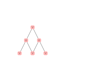
in the following game tree
- memory needed = t memory(one position)
- alternating rows in the following switch between ∃ and ∀
- p.368 it is possible to build positions in GO which encode arbitrary QSAT formulas, thus GO is PSPACE complete.
- computers recently got better at GO by searching as far as they could, and then filling open space up randomly with stones and seeing how the territory breaks out
- it seems that humans search deeply but selectively
walk sat
random walking through a 3-SAT problem
3-SAT with n variables x1, …, xn in (\(\frac{4}{3}\))n poly(n)
the following is all in the book
given a formula φ
start with a random truth assignment B
if out_of_time return "don't know"
  if B.satisfies(phi)
    then return B
  else
    choose clause C randomly from all the unsat clauses
    choose X randomly from C.variables
    flip x
    recur
no-one is able to prove that this completes through an analysis of the total number of satisfied clauses.
- proof
-
Assume φ is satisfiable, →, ∃ A s.t. A
satisfies φ. Let d(A,B) be the Hamming distance between A
and B (the number of variables on which they differ). We will
analyze the change in the hamming distance.
We'll compute the probability that δ(d) is positive or negative (i.e. closer to or further from solution) with each change. In the worst case B already agrees with A in 2/3 of the variables in C, so
- Pr[δ(d) = +1] ≤ 2/3
- Pr[δ(d) = -1] ≥ 1/3
so with 2-SAT where the above Pr's are both 1/2, it will generally take n2 steps to find a satisfying assignment (see the math-aside)
however in our case where we're more likely to move away from than towards a hamming distance of 0.
We can look at p(d) if we start at a distance of d from A, p(d) is the probability that we will ever read d=0 instead of drifting infinitely far away from the best solution.
p(d) = 1/3(p(d-1)) + 2/3(p(d+1))
left as an exercise, given the above p(d)=½n
if you will ever touch 0, then you probably will within the first O(d) steps, in fact 3d steps is generally all you need.
this is all important because we will wrap our algorithm in another outer loop. A random restart loop, which will restart our algorithm from time to time. Basically we will start over every 3n steps.
so (back to our running time), we will restart (4/3)n times and each time will take poly(n) (running 3n steps) times, then we will succeed with ¾n likelihood, so our average number of attempts will be the inverse of the probability of success.
our average value of p(d) will be… \begin{eqnarray*} P_{success} &=& \sum_{d=0}^n{Pr[d(A,B)=d]p(d)}\\ P_{success} &=& \frac{1}{2^n}\sum_{d=0}^n{{{n}\choose{d}} \frac{1}{2^d}} \\ P_{success} &=& \frac{1}{2^n}(\frac{1}{2}+1)^n\\ P_{success} &=& \left(\frac{3}{4}\right)^n \end{eqnarray*}
this is very close to the best known algorithm for 3-SAT, the best is αn with α=1.332 where as this one is α=1.333… the other one is super-complicated, and uses this as a subroutine
-
some random walk stuff (homework relevant), we should really
know this stuff
when we go left or right with equal probability after 2 steps we will be at our starting point with probability 1/2, after four steps it would be with probability 6/16
in general after t steps we could be anywhere from -t to +t from our starting point. lots of \({t}\choose{n} \times \frac{1}{2^t}\), which when graphed looks like a normal distribution around t/2 with width 1/sqrt(t).
given that n! ≅ nn e-n, (see math appendix)
math aside
Random Walk: in a random walk on n steps, starting in the middle it will take n2 steps to reach 0.
when flipping random coins the resulting number of heads will be a bell curve centered around t/2 with a width of sqrt(t).
when reporting error from a set of trials, e.g. p plus or minus ε, then ε ∼ 1/sqrt(t) where t is the number of trials.
*read the math appendix!*
2010-04-29 Thu
counting in SPACE m and NSPACE m
- stronger than TIME m
- still limited
- counting? up to 2m
we can count higher with randomness
- w/deterministic machine of m states, after 2m steps we've repeated something and are in a loop.
- w/non-deterministic machine of m states, after 2m steps it is possible that ∃ unvisited states after 2m steps
the expected time to get to any state $i$,
$$\mathbb{E}T_i = 2(\mathbb{E}T_{i-1} +1) \sim 2^i$$so with a randomized machine we can count to \(2^{2^m}\)
improved counting
using \(\mathbb{E}T_i = 2^i\) we can output an update every time we enter a previously unseen state (suppose our output screen has sufficient memory to handle this part)
- can't get better than factor of 2 accuracy
- additional "noise" due to randomness
ideas/solutions:
- changing probabilities to forward with back ¼ and forward ¾.
-
controlling variance: if we split our clock up into t pieces of
size m/t, and independently run a clock in each piece, then the
average of these clock times will be closer to the expected time.
how close will these be? we can apply chebyshev's inequality (below). ∀ clocks i, let Yi be the clock's time, then $$ Pr\left(\left|\frac{y_1, \ldots, y_t}{t}\right|-\mathbb{E}y_i \leq t\sqrt{Var\left(\frac{y_1, \ldots, y_t}{t}\right)}\right) \leq \frac{1}{t^2} $$
definition of variance, \(var(x) = \mathbb{E}((x - \mathbb{E}x)^2)\), expected distance from average value, squared
- if x is a coin flip
-
\(\mathbb{E}x=\frac{1}{2}\)
- \((0-\frac{1}{2})^2 = \frac{1}{4}\)
- \((1-\frac{1}{2})^2 = \frac{1}{4}\)
-
2 coins, x and y
- \(\mathbb{E}(x+y)=1=2\mathbb{E}(x)\)
- Var(x+y)=1/4*(-1)2+1/2*02+1/4*12=1/2=2Var(x)
- \((Var(x+y))^{\frac{1}{2}}=2^{\frac{1}{2} \times (Var(x))^{\frac{1}{2}}}\)
- so with k flips, the expectation grows by a factor of k, and the variance grows by a factor of \(k^{1/2}\)
Chebyshev Inequality: ∀ t ≥ 0, \(Prob(abs((z-\mathbb{E}(z))) \geq t\sqrt{Var(z)}) \leq \frac{1}{t^2}\) Law of Large Numbers: independent random variables, x1, x2, x3, …, the limit of the average value will converge to the expected value, also stated as $$ lim_{t \rightarrow \inf}{\frac{x_1+x_2+\ldots+x_t}{t}}=\mathbb{E}x $$ 2 facts:
- ∀ x, 1-x ≤ e-x
- ∀ x, 1+x ≤ ex
application to streaming algorithms
Alon, Matias, Szegedy 1996 – approximating frequency moments
you have some vast amount of stuff (say google web searches) flying past you, and you just want to update a couple of bits as these gigs fly by.
stream of numbers from the set {1, …, N}, and we want an idea of the number of distinct elements in the stream (the 0th frequency moment)
- mi = # times i appears in the stream
- the kth frequency moment $$F_k=\sum_{i=1}^{b}{(m_i^k)}$$
One approach for F0 (# distinct) would be to track the smallest element seen thus far.
- let J = the smallest element in the stream
- \(\mathbb{E}J=\frac{N}{F_0}\), so if J is close to its expectation, then a good estimate for F0 is \(\frac{N}{J}\)
2010-05-04 Tue
approximation algorithms
we've spent a lot of time saying how all NP-complete problems are equally hard, however when you are approximating the solutions they are not all equally hard.
branch and bound and branch and cut are popular approaches for real-world approximations of the solutions of NP-complete problems
- vertex cover
Vertex Cover- input
- a graph G=(V,E) and an integer i
- question
- what is the smallest vertex cover S ⊆ V
B is NP-hard if A ⊆ B ∀ A ∈ NP
Algorithm for a decent vertex cover
- start: S = ∅
-
while ∃ uncovered edges(u,v) s.t. (u,v ∉ S)
- add u,v to S
A is a 2-approximation for a minimal vertex cover, so $$ \frac{|S_A|}{S_{opt}} \leq 2 $$ proof: the sequence of edges covered by this method are disjoint (a partial matching), the optimal vertex cover (VC) must include at least 1 of the ends of each of these edges, or at least ½ as many vertices as included in this cover.
the kicker here is that we can't do any better than this silly algorithm for a poly-time algorithm.
- fuzzy vertex cover
one other approach for vertex cover is the following Fuzzy vertex cover; variables, ∀ v ∈ V, 0 ≤ xv ≤ 1 s.t. ∀ (u,v) ∈ E, xu + xv ≥ 1here we want to minimize the sum of the vertices in the cover rather than the number of vertices
this is called a linear programming relaxation of this problem
from the above we can get a real vertex cover in the following way; v ∈ S ↔ xv ≥ \frac1/2
this also results in a two approximation of the minimal VC
- continuously approximatable problems – Fully Poly Time Approx. Scheme (FPTAS)
∀ ε > 0, ∃ a (1+ε)-approximation that takes poly(n,1/ε) time - Traveling Salesman Problem (TSP)
Traveling Salesman Problem- input
- n by n matrix dij
- question
- tour s.t. i1, i2, …, in which minimizes \(\sum_{j=0}^{n-1}{d_{i_j,i_{j+1}}}\)
Hamiltonian Path ⊆ TSPthreshold ⊆ TSPoptimization
$$ d_{ij} = \left\{ \begin{array}{ll} 1 &: (i,j) \in E\\ 1000000 &: (i,j) \notin E \end{array} \right. $$∃ a Hamiltonian path ↔ the shortest path above has distance ≤ n
note that the above could violate the triangle inequality, or ∀ i,j,k , dik ≤ dij + djk
we can uses a minimal spanning tree (which can be found ∈ P) to build a not so bad Hamiltonian path
MSTop ≤ Topt ≤ 2MSTopt
The above uses the triangle inequality when short-circuiting a tour along the MST, by skipping previously visited cities.
traveling out and back on all edges in MST (doubling the edges into a multipath) leads to an Eulerian tour. ∃ an Eulerian tour ↔ each vertex has even degree, we can force each edge to have even degree by only adding edges between vertices which have odd degree – this is a more efficient way of generating a shortest tour (TB) from an MST
TB ≤ MST + MM ≤ 3/2 Topt – where MM is the minimum matching of the odd degree vertices
Euclidean TSP (1+ε)-approximation in \(\sim n^{\frac{1}{\epsilon}}\) -- done w/dynamic programming
2010-05-06 Thu
Quantum Mechanics
- The "two slit" experiment
performable with waves of light or water.- Light of some frequency hits a screen with two holes in it, and then hits a second screen on the other side of the first screen.
- the light propagates from each hole at some new frequency
- at different points in the second screen the two lights will either arrive in phase, or out of phase with each other – as a result the light on the second screen appears at a higher frequency than the original waves of light
in the late 1800s this experiment was carried out with very faint light sources – such that small numbers of individual particles should be hitting the back screen, however the continuous wave effect was surprisingly still observed.
similarly this experiment has been performed with the light replaced with single electrons passing through the slit screen at a single time, and the single electron lands on the screen with the exact sum of the probabilities of moving through both slits.
so rather than probability the amplitude of arriving on the second screen at some point is the sum of the amplitudes (measured in complex numbers) of the electron moving through each slit.
$$ probability = \sum|amplitude|^2 $$some funny facts – placing a detector on the slits which detects which of the slits the electron have moved through, then the results on the back screen do not show the sum of amplitudes of both slits but rather only of the detected slit. This is due to decoherence when the actual measuring of the electron is intricately linked with the remainder of the universe.
- quantum computing
due to decoherence it is necessary to both bind some states of the computing elements in such a way that they are not truly random, but such that stray electrons moving by the computer don't bounce off an element and inadvertently measure its state thereby removing its quantum state.the above may be harder than landing on Mars but easier than constructing a space elevator.
physics at the microscopic level is reversible, meaning the machine code level operations may also need to be reversible (i.e. ⊕ instead of ∧).
- quantum operations
computational state changes through reversible matrix multiplication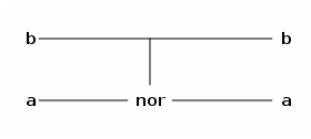
nor applied to a and b $$ \left( \begin{array}{llll} 1 & 0 & 0 & 0\\ 0 & 0 & 0 & 1\\ 0 & 0 & 1 & 0\\ 0 & 1 & 0 & 0 \end{array} \right) \left( \begin{array}{llll} 1 & 0\\ 0 & 1\\ 1 & 0\\ 1 & 1 \end{array} \right) $$ if our computer is represented as a large vector of bits
an example quantum operator $$ \frac{1}{\sqrt{2}} \left( \begin{array}{lr} 1 & 1\\ 1 & -1 \end{array} \right) \left( \begin{array}{l} 1\\ 0 \end{array} \right) = \left( \begin{array}{l} \frac{1}{\sqrt{2}}\\ \frac{1}{\sqrt{2}} \end{array} \right) $$ the above applied to $$ \left( \begin{array}{l} \frac{1}{\sqrt{2}}\\ \frac{1}{\sqrt{2}} \end{array} \right) $$ yields $$ \left( \begin{array}{l} 1\\ 0 \end{array} \right) $$ and applied to $$ \left( \begin{array}{l} \frac{1}{\sqrt{2}}\\ -\frac{1}{\sqrt{2}} \end{array} \right) $$ yields $$ \left( \begin{array}{l} 0\\ 1 \end{array} \right) $$
- reversible computation
every erased bit must result in some generation of heat (entropy), however reversible computation need not theoretically generate heat - example quantum computation
f:{0,1} → {1,0}, is f(0) == f(1)?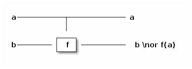
you can in effect run f on 0 and 1 at the same time with
- a = 1/sqrt(2)(0+1)
- b = 1/sqrt(2)(0-1)
the following is true if f(0)==f(1) $$ \frac{1}{2} \left( \begin{array}{rr} 0 & 0\\ -0 & 1\\ 1 & 0\\ -0 & 1 \end{array} \right) \rightarrow \left( \begin{array}{r} -\frac{1}{2}\\ \frac{1}{2}\\ -\frac{1}{2}\\ \frac{1}{2} \end{array} \right) $$ we don't know what the values are, but we can play tricks with interference to find out if they are the same value
aside from all these artificial problems, we found out that factoring was qualitatively different on quantum computers
- quantum factoring
want to factor N=pq where p and q are prime, let n=log(N) – or the bits required to store N- choose a random c∈{2, …, N-1}
- if gcd(c,N) ≠ 1 then we're done
- else compute powers of c, mod n: and find the order of c or the smallest r s.t. cr = 1 – this is the period of this sequence
- if r is odd then start over
- else r is even
- cr ≡ 1 mod n → cr-1 is a multiple of N, ∃ k s.t. cr-1=kn, since r is even we can do \((c^{\frac{r}{2}}-1)(c^{\frac{r}{2}}+1)=kn\)
- now we compute the \(gcd(c^{\frac{r}{2}}-1, N), gcd(c^{\frac{r}{2}}+1, N)\)
- if one of these is a multiple of N, then try again, else done
do the above a small number of times and you will win
the only thing here that can't be done in poly time is finding the order of c mod n, which could take exponential time
on a quantum computer we
- put a register x into a superposition of all possible values from 0 to N.
- have an empty register set to 0
- we run a program which computer cx mod n, and feed it our super-positioned x, and compute cx mod n for all of these values.
-
we now measure the output of this program, when we measure one
particular output the wave function collapses in x, and everything
that doesn't map to that particular output falls to 0.
x is now in a periodic state, and r is the period of this state
we can take the Fourier transform of x to find its period, this can be done in O(log2(N)) quantum steps
misc
giving a good colloquial talk
terms
- simple graph
- every pair of vertices share at most 1 edge
- turing reduction
- A \(\leq\) B if A can be solved with a polynomial number of calls to B
- karp reduction
- A \(\leq\) B if each instance of A can be converted to an instance of B s.t. yes(A) iff yes(B)
- CNF
- conjunctive normal form conjunction of clauses each of which is a disjunction of literals
- linear programming
- a programming problem where the goal is to minimize some linear combination of a series of vertices (see fuzzy-vertex-cover)