Software Foundations 558
-
Office Hours:
- Tue: 10:00 - 11:00
- Thu: 12:15 - 1:15
- http://digamma.cs.unm.edu/~darko/classes/2009f-558/index.html
- syllabus.pdf
Table of Contents
- meta stuff
- class notes
- 2009-08-25 Tue [2/2]
- 2009-08-27 Thu
- 2009-09-01 Tue
- 2009-09-03 Thu
- 2009-09-08 Tue
- 2009-09-10 Thu
- 2009-09-17 Thu
- 2009-09-22 Tue
- 2009-09-24 Thu
- 2009-09-29 Tue
- 2009-10-06 Tue
- 2009-10-08 Thu
- 2009-10-13 Tue
- 2009-10-20 Tue
- 2009-10-22 Thu
- 2009-10-27 Tue
- 2009-10-29 Thu
- 2009-11-03 Tue
- 2009-11-05 Thu
- 2009-11-10 Tue
- 2009-11-12 Thu
- 2009-12-01 Tue
- 2009-12-03 Thu
- 2009-12-10 Thu
- questions / topics
meta stuff
optional reading
- Programming in Haskell can read in one sitting, intro to prog
- Introduction to Functional Programming part math, part prog more in depth, prove correctness etc…
- Practical Foundations for Programming Languages online notes, can serve as alternative to textbook
- Programming Language Pragmatics undergrad PL and compiler textbook
- Real World Haskell Orielly, in case we actually wanted to write real programs in Haskell
homework hand in
Turn In
- There is a turn-in mechanisms through cssupport.
- electronic through CS machines (need cs account)
class notes
2009-08-25 Tue [2/2]
- intro to Haskell
-
start with core of lambda calculus and begin adding features
- OO
- imperative
- most features of current programming languages
- possibly more
- [X] sign up for mailing list
- [X] get text book
2009-08-27 Thu
sum integers
C: creates the location sum in memory, then modifies it 11 times
sum = 0;
for (i=1, i<11, 1++)
  {
    sum = sum + 1;
  }
Haskell: no store, initialization, variables, etc…
sum [1..10]
sum over all integers in Haskell
sum [0..]
QuickSort
let f [] = []
let f (x:xs) = f ys ++ [x] ++ f zs
        where
          ys = [a | a <- xs, a <= x]
          zs = [b | b <- xs, b > x]
this is much clearer in functional language, but would be difficult to specify an in-place QuickSort. see "persistent data structures v.s. ephemeral data structures" for more on this
expressions
Prelude: contains basic mathematical expressions (sqrt, +, etc…), and is located in Prelude.hs
common functions in the prelude
Prelude> head [2,3,5,1]
2
Prelude> tail [2,3,5,1]
[3,5,1]
Prelude> [2,3,5,1] !! 2
5
Prelude> take 3 [2,3,5,1]
[2,3,5]
Prelude> drop 3 [2,3,5,1]
[1]
Prelude> length [2,3,5,1]
4
Prelude> sum [2,3,5,1]
11
Prelude> product [2,3,5,1]
30
Prelude> [1,2,3] ++ [2,3,5,1]
[1,2,3,2,3,5,1]
Prelude> reverse [2,3,5,1]
[1,5,3,2]
function application
- in Java f(x)
- in math f(x)
- in Haskell f x
f x + b -> f(x) + b
style in Haskell is to minimize parenthesis
Curried functions
functions always take a single argument, so in take 2 [2,5,3]
the portion take 2 returns a function which is then applied to the
list.
f x y -> (f(x))(y)
2009-09-01 Tue
technical questions
undefined is a valid token in Haskell code.
Prelude> undefined
*** Exception: Prelude.undefined
if your guards for a function don't cover some argument, then the result for that argument is undefined
fact n
    | n >= 1 = n * fact(n - 1)
    | n == 0 = 1
-- is equal to
fact n
    | n >= 1 = n * fact(n - 1)
    | n == 0 = 1
    | n < 0  = undefined
write all function definitions in files
more Haskell features / syntax
-
when you want to use a curried function infix, then you must
surround it in back quotes
average xs = sum xs `div` length xs
-- or
average xs = div (sum xs) (length xs)
-
all names (functions, variables) must start with lower-case letters
funny ns = sum ns + length ns
-- or
funny ns = (+) (sum ns) (length ns)
- indentation matters, code is 2-D (like python), however there are 1-D options for all expression, and in fact these 1-D options are the basic or core of Haskell which the complex 2-D layout stuff is translated to.
-
the
!!notation is used to index into a list -
comments
-
single line starts with
-- -
multi line functions use
{--}notation
-
single line starts with
types
- can be explicit about types
-
::means has the type -
all types are capitalized
False :: Bool
'5' :: Char
5 :: Int
"a" :: String
"a" :: [Char]
[False, True] :: [Bool]
we will use type declarations for every function which we will write
types
- Int
- machine size integers
- Integer
- integers of arbitrary size
- Float
- numbers with decimals
- Bool
- boolean
- Char
- characters
- String
-
is the same as a list of characters
[Char]
uppcase :: String -> String
uppcase str = map f s
    where
      f :: Char -> Char
      f 'a' = 'A'
      f 'b' = 'B'
...
      f c = c
reference
- http://haskell.org contains the prefix etc…
- hoogle provides a search through haskell
2009-09-03 Thu
question: executable with main
module Main where
    fac 0 = 1
    fac n = n * fac(n - 1)
    main =
        putStrLn "hello"
types
[False, False] :: [Bool]
[1..] :: [Integer]
- tuple
-
is like a record, can contain multiple values of different
types. tuples can be any size but it's size if fixed.
(False, True) :: (Bool, Bool)
(False, 'a', 1) :: (Bool, Char, Int)
div 5 9-
-
div 5returns a function which divides 5 by it's argument. the type of div isdiv :: Integer -> (Integer -> Integer)
-
->-
we just say that the
->constructor associates to the right, so we don't have to write the parenthesis as above.
by having every function take exactly one argument, Haskell and ML
avoid the complexities of needing to have having apply operators
like in lisp
when passing complex arguments to functions you can use pattern matching to automatically deconstruct the complex argument
f (b,n) = b + n
- polymorphic functions
-
can take multiple types of arguments
length :: [Integer] -> Integer
-- or
length :: [Char] -> Integer
- type variables
-
can be used to represent multiple types
length :: [a] -> Integer
-- or
take :: Integer -> [a] -> [a]
fst :: (a,b) -> a
id :: a -> a
- overloading
- when you want multiple types, but not all types you basically are overloading the function (defining it multiple times for multiple argument types)
- type classes
-
Haskell manages overloading by defining classes of
multiple types. see the prelude for type classes.
type class constraints can be placed in front of
type class constructions
product :: Num a => [a] -> a
+ :: Num a => a -> a -> a
- Num
- numerical types
- Eq
- equality types
- Ord
- ordered types
2009-09-08 Tue
pattern matching
abs :: Int -> Int
abs n
    | n < 0 = -n
    | otherwise = n
not :: Bool -> Bool
not False = True
not True = False
wildcard _
(and) :: Bool -> Bool -> Bool
True and True = True
_ and _ = False
note that the above and clause is not short-circuiting, while the next one is
(and) :: Bool -> Bool -> Bool
True and b = b
False and _ = False
lazy evaluation
allows the use of infinite data structures
[1..] is the infinite list
lists use the : cons operator
[1, 2, 3]
anonymous functions lambda (written \)
(\ x -> x + 2) 4 -- is equal to 6
useful when combined with map
firstodss n = map (\ x -> x + 1) [0..n-1]
sections (partial infix operators)
shorthand for lambda extractions
-- the following are all equivalent
1 + 2
(+) 1 2
(1+) 2
(+2) 1
can be handy
map (*2) [1, 2, 3, 4]
list comprehension
[x^2 | x <- [1..5]]
-- is equal to
map (^2) [1..5]
more interesting list comprehension
-- multiple generators
[(x,y) | x < [1, 2, 3], y <- [4,5]]
-- triangular
[(x,y) | x <- [1, 2, 3], y <- [x..3]]
- concat
-
flattening function for lists
concat xss = [[x] | xs <- xss, x <- xs]
guards
[[x] | x <- [1..10], even x]
finding primes
factors n = [[x] | x <- [1..n], n `mod` x == 0]
prime n = factors n == [1,2]
primes n = [[x] | x <- [2..n], prime x]
2009-09-10 Thu
continue where we left off (more examples)
zip
combines lists
zip : [a] -> [b] -> [(a, b)]
zip [] _  = []
zip _ []  = []
zip [a] [b] = [(a,b)]
zip (a:as) (b:bs) = (a,b) : (zip as bs)
turn a list into a list of pairs
pairs [a] -> [(a, a)]
pairs xs = zip xs (tail xs)
sorted :: [Ord] -> Bool
sorted [x] = True
sorted xs = foldl (and) True (map (\ x y -> if (x < y) True else False) (pairs xs))
-- more concisely
sorted xs = [ x <= y | (x,y) <- pairs xs]
count lower-case letters in string
numlower :: String -> Int
numlower str = length [x | x < str, isLower x]
recursive list functions
product Num a => [a] -> a
product [] = 1
product (x : xs) = x * (product xs)
length :: [a] -> Int
length [] = 0
length (_:xs) = 1 + (length xs)
reverse [a] -> [a]
reverse [] = []
reverse (x:xs) = (reverse xs) ++ [x]
how fast is reverse… I'd think its O(n)
reverse [1, 2, 3]
(reverse [2,3]) ++ [1]
((reverse [3]) ++ [2]) ++ [1]
(((reverse []) ++ [3]) ++ [2]) ++ [1]
(([] ++ [3]) ++ [2]) ++ [1]
([3] ++ [2]) ++ 1
[3, 2] ++ [1]
[3, 2, 1]
++ must traverse the list, so it doesn't run in unit time, so we run
in n2 time
maybe
reverse [a] -> [a]
reverse xs = foldl (++) [] xs
concat :: [[a]] -> [a]
concat xss = [x | xs <- xxs, x <- xs]
-- or recursively
concat [] = []
concat (x:xs) = x ++ (concat xs)
replicate :: Int a -> [a]
replicate 0 _ = []
replicate n x = x : (replicate (n - 1) x)
(!!) :: [a] -> Int -> a
(x:xs) !! 0 = x
(x:xs) !! n = xs !! (n - 1)
elem :: Eq a => a -> [a] -> Bool
elem _ [] = False
elem x (y:ys) = (x == y) or (elem x ys)
What types would not be comparable? Functions
map :: (a -> b) -> [a] -> [b]
map f xs = [f x | x <- xs]
-- now recursively
map f [] = []
map f (x:xs) = f x : map f xs
filter :: (a -> Bool) -> [a] -> [a]
filter f xs = [x | x <- xs, fx]
-- recursively
filter f [] = []
filter f (x:xs)
           | p x = x : filter xs
           | otherwise = filter xs
2009-09-17 Thu
our own types, and their classes
How to define types and make them instances of type classes
In standard Haskell it is not possible to have a type which is dependent on a value.
- Type Synonym
-
do not introduce new types
type Point = (Float, Float)
- New Type
-
does introduce a new type
data Point2D = Point2D (Float, Float)
this actually does introduce a new type, which we can use
pointA, pointB :: Point2D
pointA = Point2D(2.0, 3.0)
pointB = Point2D(3.0, 4.0)
-- we can then define functions on these types
distance (Point2D(x1, y1)) (Point2D(x2, y2)) = sqrt((x1 - x2)^2 + (y1-y2^2))
the new
Point2Dsyntactic element is a tag which has the type of a function from a pair ofFloatsto the typePoint2D. It is not necessary for the tag and the type to have the same name. - types w/variants
-
a type which has multiple constructors
data Point2D = Rect (Float, Float)  -- (x,y)
             | Polar (Float, Float) -- (theta, r)
-- we can then use these types
pointC :: Point2D
pointC = Polar(2.0, 1.5)
-- and define functions
distance(Rect(x1, y1))(Rect(x2, y2))   = sqrt((x1 - x2)^2 + (y1-y2^2))
distance(Polar(x1, y1))(Rect(x2, y2))  =
distance(Rect(x1, y1))(Rect(x2, y2))   = distance(Polar(x1, y1))(Rect(x2, y2))
distance(Polar(x1, y1))(Polar(x2, y2)) =
- recursive data types
-
for real fun, we need to recurse
data BnIntTree = Leaf Int
               -- normally in haskell curried functions are prefered to tuples
               | Node BnIntTree BnIntTree
and to use said structure…
tree1 :: BinIntTree
tree1 = Leaf 1
tree123 :: BinIntTree
tree123 = Node (Node (Leaf 1) (Leaf 2)) (Leaf 3)
for more stuff…
-- lets count our leaves
countLeaves :: BinIntTree -> Int
countLeaves (Leaf n) = 1
countLeaves (Node t1 t2) = (countLeaves t1) + (countLeaves t2)
-- lets add our leaf values
addLeaves :: BinIntTree -> Int
addLeaves (Leaf n) = n
addLeaves (Node t1 t2) = (addLeaves t1) + (addLeaves t2)
-- left to right traversal
traverseTreeLeft :: BinIntTree -> [Int]
traverseTreeLeft (Leaf n) = [n]
traverseTreeLeft (Node t1 t2) = (traverseTreeLeft t1) ++ (traverseTreeLeft t2)
-- right to left traversal
traverseTreeRight :: BinIntTree -> [Int]
traverseTreeRight (Leaf n) = [n]
traverseTreeRight (Node t1 t2) = (traverseTreeRight t2) ++ (traverseTreeRight t1)
-- map some function across a tree
mapBinIntTree :: (Int -> Int) -> BinIntTree -> BinIntTree
mapBinIntTree f (Leaf n) = Leaf (f n)
mapBinIntTree f (Node t1 t2) = Node (mapBinIntTree f t1) (mapBinIntTree f t2)
-- height
heightBinIntTree :: BinIntTree -> Int
heightBinIntTree (Leaf _) = 0
heightBinIntTree (Node t1 t2) = 1 + (heightBinIntTree t1 `max` heightBinIntTree t2)
- new tree data type
-
abstract arithmetic syntax tree
data ArExp = Mul ArExp ArExp
           | Add ArExp ArExp
           | Number Num
now to evaluate said expressions
evaluate :: ArExp -> Int
evaluate (Mul e1 e2) = evaluate e1 * evaluate e2
evaluate (Add e1 e2) = evaluate e1 + evaluate e2
evaluate Number n = n
pretty print
-- just do the pattern above only construct/concat strings
2009-09-22 Tue
parameters to type constructors
another way to define Point2D
type Pair a = (a,a)
type Point2D = Pair Float
can also do this with data (remember data actually defines a new
structure while type defines something more like an alias)
data BinIntTree = Leaf Int
                | Node BinIntTree BinIntTree
-- or can be written as
data BinTree a = Leaf a
               | Node (BinTree a) (BinTree a)
type BinIntTree = BinTree Int
if we wanted to define lists
data MyList a = Empty
              | Nonempty a (MyList a)
-- to construct values of this type
list1 :: MyList Char
list1 = Nonempty 'r' (Nonempty 'e' (Nonempty '1' Empty))
lists in the prelude (same functionality, different syntax)
-- this isn't really legal haskell
data [] a = []
          | a : ([] a)
-- to construct values of this type
list2 :: [Char]
list2 = 'r' : ('e' : ('1' : []))
foldr abstract the structure or recursive list traversal
foldr is a higher order function to hold this common form
f [] = v
f (x:xs) = x (+) xs
so
sum = foldr (+) 0
product = foldr (*) 1
and = foldr (&&) True
type of foldr
foldr :: (a -> b -> b) -> b -> [a] -> b
when list is thought of as a series of cons'd lists, then foldr can be thought of as
- replacing the cons with it's function
- replacing the empty list with it's base value
-
length using foldr
length = foldr (\ _ a = 1 + a) 0
-- or more satisfyingly
length = foldr (const (1+)) 0
-
reverse using foldr
reverse = foldr (\ x r -> r ++ [x]) []
function composition
even :: Int -> Bool
not :: Bool -> Bool
-- lets use the above to define the below
odd :: Int -> Bool
odd n = not (even n)
-- even better (using function composition)
odd = not . even
this last example is an instance of the point free style of definition
to define .
(f . g) a = f (g a)
(f . g) = (\ a -> f (g a))
2009-09-24 Thu
some more higher order functions…
- map
- applies function to list
- filter
- filters list on some function
express list comprehension using map and filter
[f x | x <- xs, p x]
-- in terms of map and filter
(map f . filter p) xs -- could be point free
map :: a -> b -> [a] -> [b]
map f = foldr accum (\ x accum -> (f x):accum) []
-- or more point free
map f = foldr (\ x -> ((fx):)) []
-- can the above be simplified to eliminate all lambdas
-- my first guess
filter p = foldr (\ x -> ((if (p x) then x else []) ++)) []
-- better
filter p = foldr (\ x -> (if (p x) then (x :) else id)) []
-- if we hate if-then-else
cond p f g = if (p x) then (f x) else (g x)
filter p = foldr (cond p (:) (\ _ -> id)) []
filter p = foldr (cond p (:) (const id)) [] -- lookup const
algebra on functions like the above is an example of "eta-expansion" or "eta-reduction"
back to map
map = foldr (\ x -> ((f x):)) []
map = foldr ((:) . f) []
equational reasoning (of the map redefinition above)
for algebraic program transformation
-
first we calculate
 y
y
y: by definition (:) y by two eta expansions (\a -> \b -> a:b) by function application (beta-reduction) \b -> y:b -
in particular
\r -> fx:r = (fx:)where y is fx(\x -> (fx:)) a b by function application (fa:) b by def of sections (:) (fa) b make parenthesis explicit ((:) (fa)) b by def. of function composition (((:) . f) a) b dropping parens (: . f) a b
2009-09-29 Tue
a Haskell is a set of defining equations
lazy evaluation
(for now) use instead of meaning
- infinite list
-
(e.g.
[6..]is list of 6 to infinity). to practically use an infinite list we must only deal with some finite portion of the list, this can be done using thetakeprefix operator, or the!!index operator.-- create an infinite list of factorials factorials = map fact [0..] -- first 5 factorial values take f factorials -- factorial of 9 factorials !! 9
- w/list comprehension
-
can create infinite lists with list
comprehension
-- squares
squares = [x^2 | x <- [0..]]
-- powers of an integer
powers :: Integer -> [Integer]
powers n = [2^x | x <- [0..]]
-- using a nice build in function `iterate'
powers n = iterate (p*) 1
- iterate
-
how to write iterate
iterate :: (a -> b) -> a -> [b]
iterate f x = x : iterate f (f x)
- primes
-
primes :: [Integer]
primers = [p | p <- [2..], prime p]
    where
      prime :: Integer -> Bool
      prime n = null (nonTrivialFactors n)
          where
            nonTrivialFactors n = filter (\ x -> n mod x == 0) [2..n-1]
- so now what is this
-
it is an infinite list of infinite lists.
map powers primes- how do we access elements of this list w/o evaluating the entirety of it's predecessors?
- example
-
example working with infinite lists
ints = 1 : map (1+) ints
odds and ends
- literate programming
a program is a work of literaturecomments
-- comment
{- literate comment -}
.lhsfiles can be ingested by all Haskell compilers. These files can be constructed in the following files- Bird-style
- all text is considered to be a comment, to write code first input an empty line following by code lines prefixed with "> ", the code is then ended with another empty line
- LaTeX-style
-
main body is Latex code, to write code wrap it in a
\begin{code}...\end{code}LaTeX environment - lhs2TeX
-
this is a preprocessor for the LaTeX-style of
.lhsfiles, that can be used to make the haskell code look more like math if desired (i.e. converting -> to arrows, Greek letters to Greek, etc…).
From now on we will be required to submit our code in a literate programming style.
- fold for generic data types
Arithmetic Data Typedata Expr = Num Int | Mul Expre Expr eval :: Expr => Int eval (Num n) = n eval (Mul e1 e2) = eval e1 * eval e2 -- now to define fold for the Expr type foldExpr (Int -> a) -> (a -> a -> a) -> Expr -> a foldExpr f g (Num n) = f n foldExpr f g (Mul e1 e2) = foldExpr e1 `g` foldExpr e2 -- or using case foldExpr fNum fMul e = case e of Num n -> fNum n Mul e1 e2 -> foldExpr e1 `fMul` foldExpr e2 -- evaluating with our combining function eval = foldExpr (id) (*) eval = foldExpr (\ (Num n) -> n) (\ (Mul e1 e2) -> eval e1 * eval e2) -- printing with the combining function to_string = foldExpr show (\ s1 s2 -> "("++s1++" * "++s2++")")
note that this can be done automatically in generic Haskell (feel free to investigate extensions that provide this, but don't use them as they're not part of the standard)
using data genericity certain functions are defined automatically whenever a data structure is defined.
2009-10-06 Tue
homework/midterm grades
homework
| median | 100 |
| average | 94 |
midterm
| median | 40 |
| average | 42 |
notes/topics from homework/midterm
- homework problem 2
data Expr = Num Integer
          | Let {var :: String, value :: Expr, body :: Expr}

-- same as
data Expr = Num Integer
          | Let String, Expr, Expr
- midterm problem 1
jj where j x = j x-
type is
a -
value
diverges
f (2, [1, 2, 3])
  where
    f (n, x:xs) = f (n-1, xs)
    f (0, xs) = xs
-
type is
[Int] -
value is
fails, because eventually the list is empty and that case isn't matched (because when the list is empty n doesn't equal 0)
-
type is
- midterm problem 3
my solution which was wrong
inits [] = [[]]
inits (x:xs) = (\ rest -> rest ++ (head (reverse rest) : [x])) (inits xs)
in general on tests, you should evaluate your function by hand on a small input to ensure that the mechanics work
- midterm problem 4
keep around the depth information in the same way that you would have in C?
2009-10-08 Thu
homework questions
- question 2.2.4 (the assembler)
- turn a large string (including newlines) into a program, the large string will look like the example in 2.2.5 (i.e. the output of "the disassembler" from question 2.2.3)
the homework introduces some new concepts
- IO
- we need to learn a little bit about IO, but don't need to understand monads
-
the PRINT statements will return a type
IO()all of which must be accumulated during the course of executing the program
reasoning about functions & data structures
- pairs
(a,b)
-- take the first of a pair
fst :: (a, b) -> a
fst (x, _) = x
-- take the second of a pair
snd :: (a, b) -> b
fst(_, y) = y
- pair
-
no special function is needed to create a pair, rather the
function
pairwill be used to do something more subtle (apply a pair of functions to a value).pair :: (a -> b, a -> c) -> a -> (b, c) pair (f, g) x = (f x, g x)
- cross
-
like pair but applies a pair of functions to a pair of
values
cross :: (a -> c, b -> d) -> (a, b) -> (c, d)
cross (f, g) (x, y) = (f x, g y)
can we define
crossin terms ofpair? or course we can.cross (f, g) = pair (f . fst, g . snd)
now lets prove some properties of
pairandcross- prove
fst . pair (f, g) = f -
in the calculational proof style
-- being painfully verbose
(fst . pair (f, g)) x
== {- definition of function composition -}
fst (pair (f, g) x)
== {- definition of pair -}
fst (f x, g x)
== {- definition of fst -}
f x
we have established, by calculation, that for any arbitrary
xfst . pair (f, g) x == f x
By extensionality
fst . pair (f, g) == f
- pair exercises
- prove that
snd . pair (f, g) = g -
we know that ∀
x-- snd . pair (f, g) = g pair (f, g) x == (f x, g x) -- by the definition of pair snd (f x, g x) == g x -- by the definition of snd -- so for any x (snd . pair (f, g)) x == g x
- prove that
pair (f, g) . h = pair (f . h, g . h) -
∀
x-- pair (f, g) . h = pair (f . h, g . h) (pair (f, g) . h) x == pair (f, g) (h x) -- by the definition of (.) pair (f, g) h x == (f (h x), g (h x)) -- by the definition of pair (f (h x), g (h x)) == (f . h x, g . h x) -- by the definition of (.) (f . h x, g . h x) == pair (f . h, g . h) x -- by the definition of pair
- prove that
cross (f, g) . pair (h, k) = pair (f . h, g . k) -
∀
x-- cross (f, g) . pair (h, k) = pair (f . h, g . k) cross (f, g) . pair (h, k) x -- definition of pair == cross (f, g) . (h x, k x) --
- ???
-
prove that
cross (f, g) . cross (h, k) = cross (f . h, g . k) - ???
- what are the functions pair and cross good for?
- prove that
- laws of map
Laws ofmap-
map id = id, we must be careful here as the secondidis anidover lists -
map f . g = map f . map gso for examplemap (square . succ) [1, 2] == [4, 9]
so the left hand side of this rule is one list traversal of a complex function (
square . succ) and the right hand side is two list traversals applying two simpler functionssuccandsquare. Note that the compiler may prefer the left hand side to the right hand side because the right hand side requires 2 list traversals (time) and an intermediate data structure (space). -
map f . tail = tail . map fsomap fandtailcommute -
f . head = head . map f -
map f . reverse = reverse . map f -
map f (xs ++ ys) = map f xs ++ map f ys -
map f . concat = concat map (map f)
-
- filter
-
filter p . concat = concat . map (filter p) -
filter p . filter q = filter (\ x -> p x && q x)
-
- typing exercise
what are these types?map (map square) -- [[1, 2], [3, 4]] -> [[1, 4], [9, 16]] -- what is the type of this equation? -- we need to know the type of square map (map square) :: [[Int]] -> [[Int]] -- and map square :: [Int]
map map :: [a -> b] -> [[a] -> [b]]
to explain the above just cram the entire type of
mapinto the(a -> b)portion of the type of map
2009-10-13 Tue
Depak is lecturer
unification
Unification (or equation solving or constraint solving) this topic comes from Heibrand's PhD thesis – proving first order predicate calculus is complete – then "rediscovered" by Pravitz and Robinson (resolution principle, initially exponential algorithm, eventually quadratic, by others down to n log(n) or n α(n)).
- α(n)
- inverse of the Ackerman function
Universe
- constants
- variables
- function symbols (making no assumptions of properties)
- terms/expressions (combination of the above)
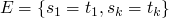
given finite set of simultaneous equations (composed of terms) we will
- determine if solvable (or unifiable), if ∃ a substitution σ (values for variables) s.t. when the variables are applied they become equal (unifier)
- if so find the most general solution (most general unifier)
possibilities
- not solvable
- solvable with single solution
- solvable with ∞ solutions
depending on the nondeterministic choices (which equation/variable to solve first) it is possible (in the case of ∞ solutions) to arrive at syntactically different solutions which will still be equivalent.
operations on the system of equations must be both
- sound
- no operation adds new solutions
- complete
- no operation removes possible solutions
basically you should be operating equally on either side of the equality relation in the equations
solvability when dealing with terms and expressions
No Solutions
-
 two functions which are not equal
-
 two functions which are not equal
-
 can't be equal as
 xis on both sides
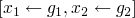
Solutions
-

-

-

-
 solvable iff
 is solvable
unification algorithm
at every point the state of the system will include
 | set of equations |
 | partial solution |
at each step there are two possibilities
- no solution if "function clash" (2 above) or "occurs check" (3 above)
-
can progress by removing equations from system and possibly adding
terms to the partial solution
-
can remove equation of the form
-
can remove equation of the form and add
 to partial solution
-
you have like 2 in the solutions above and add
 to the partial solution
- you have case 4 above in the solutions section
-
can remove equation of the form
2009-10-20 Tue
when checking whether a program has a type we will be implementing unification-type algorithms
thus begins the second part of the course
- from textbook
- more interactive
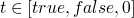
t ::=
  true
  false
  if t then t else t
  0
  succ t
  pred t
  iszero t
-
in the above
tis a place holder for any term - the above is shorthand for an inductive definition of a set of terms
- context free grammars define sets of strings
- the above defines terms (tree-like structures) rather than strings, these kinds of grammars may be called abstract grammars, as opposed to the context free grammars which are concerned with the string representations of the programs as written by the programmer
- for now we won't worry about the parsing issues, but only with the abstract trees
type systems will help to divide terms into those that are definitely meaningless and those that might have meaning
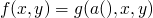
the standard notation for these inductive set definitions of the form
if  then
then  is
is

a more concrete method of constructing the set of terms


then applying these rules
- S0 = empty-set
- S1 = {true, false, 0}
- S2 = …
from syntax to semantics
evaluation is moving from sets of terms to sets of values
-- terms
t ::=
  true
  false
  if t then t else t

-- values
v ::=
  true
  false
evaluation rules
-
if true then t1 else t2
 t1
t1
-
if false then t1 else t2 t2
-
2009-10-22 Thu
homework2 notes
- definitely use LaTeX, lhs, etc…
- include test code in the resulting pdf
- include discussion in the resulting pdf
- consider effort on part of the reader/grader
- could even include the test log into the resulting pdf file
- need to be able to print a single pdf file
- minimum font is 11pt
-
use the following LaTeX font
\usepackage{mathpazo} - don't use ellipses in a proof
- don't use a narrative style in a proof (as much as possible the proof should be a system of equations)
- these calculational proofs are intended to be mechanically checkable (in style at least if not in practice)
here is an example .lhs file excerpt-CircuitDesigner.lhs
current homework notes
- we can use our own types if we prefer
- fail with cycle is just an occurs check failure
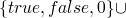
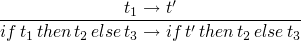
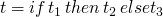
operational semantics
-
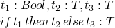
if t1 then t2 else t3is strict int1(meaning it must be known/evaluated) but is lazy int2andt3in that they may not be evaluated -
rules for if/then/else
-
(E-IFTRUE)

-
(E-IFFALSE)

-
(E-IF)
-
(E-IFTRUE)
-
repeat evaluation
->*is the transitive, reflexive closure of the single-step evaluation relation - the normal form of a term is what it ultimately evaluates to
actually stepping-through/evaluating a program
-


- …
- …
-

now adding numbers to our simple boolean language
sadly we now have normal forms that we don't like, for example
iszero false. Adding a type system to our system will allow us to
find these stuck situations before evaluating.
- well typed
- evaluation will not result in a stuck term
2009-10-27 Tue
homework2 back today average score is ~90
recall the language of arithmetic expressions
t ::= true
      false
      if t then t else t
      0
      succ t
      pred t
      iszero t
inductive function definition examples
- size
-
returns the "size" of a term
size true  = 1
size false = 1
size 0     = 1
size (succ t)   = 1 + size t
size (pred t)   = 1 + size t
size (iszero t) = 1 + size t
size (if t1 then t2 else t3) = (size t1) + (size t2) + (size t3)
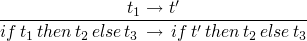
- consts
-
returns the set of constants present in a term
consts 0 = [0]
consts true = [true]
consts 0 = [false]
consts (succ t) = consts t
consts (pred t) = consts t
consts (iszero t) = consts t
consts (if t1 then t2 else t3) =
    consts t1 `union` consts t2 `union` consts t3
Theorem
- by induction on the structure of t
-
base cases are
 :
:
-
-
inductive size
-
 :
:
-
-
-
-


Operational Semantics
what if we want to describe a language on booleans where both cases of the conditional are evaluated and in addition we'd like to fix the order of evaluation to t2 then t3 then t1?
| E-IF-THEN | 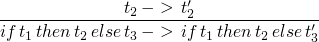 |
| E-IF-ELSE T |  |
| E-IF-ELSE F | 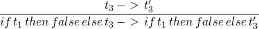 |
| E-IF-GUARD TT | 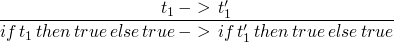 |
| and three more | … |
| E-TRUE TT |  |
| and eight more | … |
we should really have a metavariable v over values
| E-IF-THEN | |
| E-IF-ELSE | 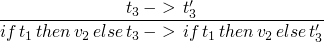 |
| E-IF-GUARD | 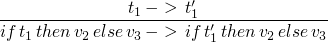 |
| E-TRUE |  |
| E-FALSE |  |
Lets type our language of arithmetic
the goal here being to eliminate normal terms which are not values
(e.g. succ(false)).
we'd prefer types to be a relation rather than a partition, so that terms can have multiple types (e.g. 1 is a natural number and an int.)
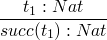
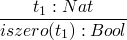
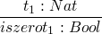
: will be our type assignment operator t:T mean t has type T
T := Nat
     Bool
rules for values


now rules for compound terms

2009-10-29 Thu
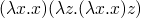
lambda calculus – there are only functions and function definitions.
what special things can you do in a language where you know that all terms will terminate
lambda calculus
 t ::= x
       \x . t
       t t
Reduction rule –  -reduction rule
- will not get more than one normal form
- is possible to end up in an infinite re-write loop
-
normal order strategy – always work with the outermost redex
-
-
call by name strategy – don't dive into a lambda
-
-
call by value – only values can be substituted into a lambda
(abstractions are considered to be values)
-


note that the two previous strategies result in different normal forms and define different lambda calculi. call by name can vaguely be thought of as a strategy in which parts of the program are set aside which can be compiled into machine code (because they won't serve as data at any point). call by name is the flavor of lambda calculus which lives in the core of Haskell – with the addition of laziness which makes it call by need.
- call by need
- haskell
- call by value
- java, C, ML, etc…
from here on out we will restrict ourselves to the call by value form of lambda calculus
untyped, call-by-value,  -calculus
terms
t ::= x
      \x . t
      t t
values
v ::= \x . t
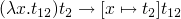
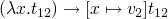
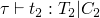
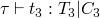
evaluation relation
- E-APPABS
-
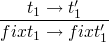
staging rules
- E-APP1
-

- E-APP2
-

tricky spot (what does  mean): which only means free
occurrences of
mean): which only means free
occurrences of  should be replaced. free terms mean those which
are not inside of a term.
should be replaced. free terms mean those which
are not inside of a term.
2009-11-03 Tue
the next homework will be out soon…
lambda calculus (Church constants)
-
 – true
-
 – false
the above are like conditionals
- true A B –> A
- false A B –> B
Church could not discover an encoding of the predecessor function, it was discovered by Fellini while he was having a tooth extracted.
– Legend
-
 – and
– and
y combinator
om = (\x -> x x)(\x -> x x)
results in
Occurs check: cannot construct the infinite type: t = t -> t1
Probable cause: `x' is applied to too many arguments
In the expression: x x
In the expression: (\ x -> x x) (\ x -> x x)
 never converges, it has no normal form
2009-11-05 Thu
formal definition of our lambda calculus / notation
very formal definition of λ-terms
-
infinite sequence of expressions called variables:

- finite, infinite or empty sequence of expressions called atomic constants which will be different from variables. (if there are none of these we have a pure λ calculus)
given the variables and atomic constants we will define λ terms
- all variables and atomic constants are λ terms and we will call these atoms
- if M and N are λ-terms, then (M N) is a λ term, this term will be called an application
- if M is a λ-term and x is a variable, then (λ x . M) is a λ term, this term will be called an abstraction
Notation
- Capital letters will denote arbitrary items
- Letters will denote variables
Parenthesis will be omitted as follows
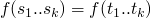
-
MNPQdenotes(((MN)P)Q) -
λ x . P Qdenotes (λ x (P Q)) -
λ x_1 x_2 ... x_n . Mdenotes(λ x_1 .(λ x_2 . (... (λ x . M) ...)))
definitions
P,Q λ-terms
P occurs in Q, or P is a subterm of Q, or Q contains P
inductive definition:
- P occurs in P
- if P occurs in M or in N, then P occurs in (MN)
- if P occurs in M or P==x, then P occurs in (λx.M)
Exercise:
-
((xy)(λx.(xy)))
- three occurrences of x
- two occurrences of (xy)
-
(λxy.xy)
- only one occurrence of (xy)
scope
- Def
- for a particular occurrence of λx.M in a term P, the occurrence of M is called the scope of the occurrence of λx.
- Example
-
in P==(λy.yx (λx.y(λy.z)x))vw
- the scope of the leftmost λy is yx (λx.y(λy.z)x
- the scope of λx is y(λy.z)x
An occurrence of a variable x in a term P is:
- bound if it is in the scope of a λx in P
- bound and binding if it is the x in λx
- free otherwise
bound and free in a term
- x is a bound variable of a term P if x has at least one binding occurrence in P
- x is a free variable of a term P if x has at least one free occurrence in P
- FV(P) is the set of free variables of the term P
- the term P is closed if it has no free variables
2009-11-10 Tue
homework notes
- is there something more elegant than string comparison for the highlighting? yes – there is an easier way if the function understands what the highlighting means
- when asking questions we should employ the phrasing "why is _ _"
-
scanning should happen in two phases
- all identifiers taken to be identifiers
- see if these presumed identifiers are identifiers or if they are keywords
- although we may not alter/remove the given function, we may create our own additional functions
-
note that the parenthesis are part of the grammar and must be
included (the same is true of
elseandtermfor theifconstruct) - the only place we really have leeway is in our acceptable identifiers
- we don't want to return any identifiers to the parser
formal definitions
- substitution
-
for any M,N,x we define [N/x]M to be the result of
substituting N for every free occurrence of x in M, and changing
bound variables to avoid clashes. other notations include:
-
[x
 N]M
N]M
- [x/N]M
- [N/x]M
-
[x
- induction on M
-
a number of rules
- [N/x]x == N - [N/x]a == a \forall atoms a != x
- [N/x](PQ) == ([N/x]P [N/x]Q) - [N/x](λx.P) == (λx.P)
- [N/x](λy.P) == (λy.P) if x $\not\in$ FV(P) - [N/x](λy.P) == (λy.[N/x]P) if x [[file:ltxpng/cs558_4ba518990fcebbf250a11f22405cb5524f2873a3.png]] FV(P) and y [[file:ltxpng/cs558_ecd413eb6f6a9015a9e6d75f9cc2e3455fd2eb4b.png]] FV(N)
-
[N/x](λy.P) == (λz.[N/x][z/y]P) if x
 FV(P) and y FV(N) where z "is fresh"
2009-11-12 Thu
homework5
simple extension of homework4, λ calculus with reductions etc…
language of Booleans and Numbers
- avoiding non-meaningful(untyped) normal terms
-
terms which do have types/meaning will evaluate and will do so
to their type
we would like to find types w/o evaluating the term, so what do we do?
- type checking should be guaranteed to terminate
- should be quick (not so true in ML or Haskell)
new syntactic type
T ::= Bool
      Nat
type of our syntactic elements
- true : Bool
- false : Bool
- 0 : Nat
-

-

-
-
so the typing system will exclude many terms which would evaluate w/o problem
goals
- well typed term will not get stuck, meaning it can be further evaluated or it is a value
- Preservation is the property that a well typed term will not evaluate in a single step to an untyped term
- Canonical forms lemma: if B has type Bool then it is either True or False
2009-12-01 Tue
homework
- many people's fresh variables weren't generating truly fresh variables
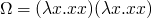
- overuse of isValue function
- average grade is around 70
Chapter 12 introduces a fixed point combinator which will allow recursion and make the language much more usable. this is done by removing the limitation of the inability to recur in the typed λ-calculus because combinators have no type (may not terminate).
lecture
would be nice to have…
- let bindings
- which are equivalent to function applications
- pairs, tuples, records
- which can also be nicely typed
2009-12-03 Thu
getting back the midterms
- typing went well
- some evaluation uncertainties
- class average 216
- look up the normal order reduction solution in the book
-
in cases where a rule has no predicates like
E-APPABS we can write the derivation tree sideways for clarity
- initial expression : (λx. (λz. λx. x z) x) (λx.xx)
- applying E-APPABS : [x |-> λx. x x] ((λz. λx. x z) x)
- resolving application : (λz. λx. x z) (λx. x x)
- applying E-APPABS : [z |-> λx. x x] (λz. λx. x z)
- resolving application : λx. x λx. x x
-
I'm not going to latex this one out…
- Nat -> Nat -> Nat != (Nat -> Nat) -> Nat, because the convention is that -> associates to the right
λ-calculus
(bridging the gap between core λ-calculus and what we need in a language)
so far we have talked about
- pairs
- tuples
- records
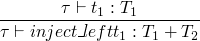
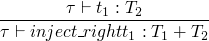
Today we will talk about variant types
when several types are all injected into a single type with labels --
these are like the data types in Haskell
T ::= T+T
t ::= inject_left t
inject_right t
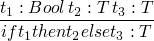
case t of { inject_left x => t | inject_right x => t }
or in Haskell
data T = A T1 | B T2

x1 :: T1
x1 = ...
x2 :: T2
x2 = ...
t1 = A x1
t2 = B x2

-- using these types
case t3 of
  A x1 -> ... x1 ...
  B x2 -> ... x2 ...
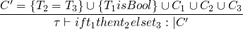
typing rules
and also a much longer one for the case rule

in our Haskell implementation of this concept we will have no idea
what T2 will be for an expression like inject_left x where x has
type T1, so we may have to force the programmer to type annotate
these expressions s.t.
-
inject_left xbecomesinject_left x as Nat x T2 -
inject_right xbecomesinject_right x as Nat T1 x
and the rules above must be changed similarly
the data keyword in Haskell introduces both the records and
variant types that we have discussed thus far as well as recursive data types which we will not have time to address this year.
recursive evaluation (in 4 minutes)
fact n in the λ-calculus
we can't say
fact n = λ n. if n == 0 then 1
                        else n * fact (n - 1)
but in λ-calculus the fact above doesn't refer to the fact being
described
λf. λn. if n == 0 then 1
                  else n * fact (n - 1)
so we end up saying…
fact = Y (λf. λn. if n == 0 then 1
                            else n * f (n - 1))
where Y is some Y-combinator, however we can't write this in our
type system, so we must add the new syntactic form fix s.t.
t ::= fix t
with typing rule
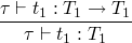
and the evaluation rules

so to perform the factorial of 6 we could do…
   (fix  (λf. λn. if n == 0 then 1
                            else n * f (n - 1))) 6
as these expand the fix(...) is inserted in place of fact in such
a way that the exposed λ-expressions are applied to their arguments
(initially 6) on every other step, and every other-other step the
fix substitution will take place. basically it alternates between
expanding and applying.
2009-12-10 Thu
type reconstruction algorithm
typing rules are similar to the evaluation rules, but in addition to requiring assumptions about the evaluation of subterms, there may also be type constraints generated during the subterm evaluation.

first, constraints C1, C2, and C3 are generated while evaluating the portions of the if statement, and two new constraints are added which are required by the if statement.
for a simpler typing constraint

while running a type constraint algorithm we will occasionally need to generate a fresh type variable which has no constraints (e.g. when calculating the type constraints on an application).
more formally the above fresh type variable creation requires a
slightly more complicated stating that the new variable (say X) is
not an element of any of the existing sets of variables used in our
subexpressions.
one valid output of our type reconstruction is polymorphic functions. one possible problem of polymorphic functions is the potential for them to be applied to different values.
for example
let id = λn.n in
(id (λk.k)) (id 5)
id is used here with different types.
the work around for this issue – discovered during the implementation of ml – is called let polymorphism and involves calculation of polymorphism during the evaluation of a let-bound. so while the above would work the following previously equivalent expression would be rejected
(λid.((id(λk.k))(id 5)))(λn.n)
what we haven't covered
- meta-theory
- analysis/proofs of the properties and relationships of/between our types and terms
- lanuage extensions
-
we skipped many possible extensions
- references
- clean way of adding mutable state to a core λ calculus
- exceptions
- chapter 14, models for raising and handling said
- subtyping
- type classes – complex interactions with type reconstruction, fundamental to Object Oriented programming. Type classes in Haskell have nothing to do with subtyping
- recursive types
-
this is not hard, but we didn't cover it.
here's a quick introduction to recursive types in Haskell.
data Tree = Leaf | Fork Tree Tree
If we think of types as sets of possible tokens, then we can recursively build the set(type) of type
Tree. Chapters 20 and 21 discuss how we can handle recursing into types. - universal polymorphism
- system F, module system, existential polymorphism
- some really interesting stuff
-
quantification over terms and
types
- dependent types
- types over types
questions / topics
BFS
Note the solution shown earlier today actually correct, the following does work however
data Tree a = Leaf a
            | Fork [Tree a]

tree = (Fork [(Fork [(Leaf 1), (Fork [(Leaf 2), (Leaf 3)])]), (Leaf 4)])

dfs :: Tree a -> [a]
dfs (Leaf l) = [l]
dfs (Fork ts) = foldr (\ t rest -> dfs t ++ rest) [] ts

-- fixed version -- Thanks to Sunny
bfs :: Tree a -> [a]
bfs (Leaf l) = [l]
bfs (Fork []) = []
bfs (Fork xs) = (concat (map bfs ([y | y <- xs, isLeaf y])))++(bfs (Fork (collapseForks [y | y <- xs, not (isLeaf y)])))
       where
               isLeaf :: Tree a -> Bool
               isLeaf (Leaf l) = True
               isLeaf _ = False
               collapseForks :: [Tree a] -> [Tree a]
               collapseForks [] = []
               collapseForks ((Fork a):xs) = a++(collapseForks xs)

tree = (Fork [(Fork [(Leaf 1), (Fork [(Leaf 2), (Leaf 3)])]), (Leaf 4)])

-- from George
bfs (Fork xs) = concatMap bfs ([y | y <- xs, isLeaf y] ++ [Fork (collapseForks [y | y <- xs, not (isLeaf y)])])
bfs (Fork xs) = [l | Leaf l <- xs] ++ bfs (Fork (concat [ts | Fork ts <- xs]))

-- broken version -- don't use
bfs :: Tree a -> [a]
bfs (Leaf l) = [l]
bfs (Fork ts) = foldr ((++).bfs) [] ([y | y <- ts, isLeaf y] ++ [y | y <- ts, not (isLeaf y)])
    where
      isLeaf :: Tree a -> Bool
      isLeaf (Leaf l) = True
      isLeaf (Fork ts) = False
Haskell IO
a list of IO actions
todoList :: [IO ()]

todoList = [putChar 'a',
            do putChar 'b'
               putChar 'c',
            do c <- getChar
               putChar c]
processes the IO actions with
sequence_ todoList
Haskell source code
partial lists
Haskell has three types of lists, finite, infinite, and partial
a partial list has an undefined final element
a = [1, 2, 3, undefined]
null operator
take a look at null
Array
create and access an array
squares = array (1,10) [(i, i*i) | i <- [1..10]]
-- then to get at a value
squares!2
Monads
- http://www.haskell.org/tutorial/monads.html
- http://en.wikipedia.org/wiki/Search?search=Monadsinfunctionalprogramming
definition (outside Haskell)
- monad
- a term for God or the first being, or the totality of all being
There are many decent monad tutorials on haskell.org. I like Wadler's tutorial from the 1995 Advanced Functional Programming summer school.
Macros, Meta-Haskell
they exist, but are different than in lisp (see meta-haskell.pdf)