|
: Self-Organizing Maps : The Fun Stuff :
: The next visualization I typically do is to simplify
the U-matrix into a
: median distance matrix. I'll use this map again in a minute to illustrate
: the significant boundaries between clusters (i.e. which dimension
contributes
: most, and in what way, to the separation of clusters).
: >> colormap(gray);
: >> U = som_umat(sMap); Um = U(1:2:size(U,1),1:2:size(U,2));
: >> h=som_cplane(sMap,Um(:)); set(h,'Edgecolor','none'); hold
on
: >> som_grid(sMap,'Label',sMap.labels,'Labelsize',10,...
: >> 'Line','none','Marker','none','Labelcolor','r'); hold off

som_distanceMatrix.gif
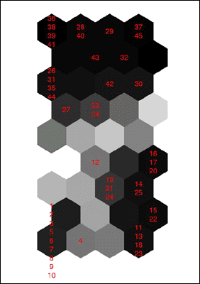
: Here we can again very clearly see the three clusters.
I've cheated a bit
: here and labeled each map node with the indices of the input vectors
which
: are closest to it in space. You'll recall that cluster 1 was vectors
no. 1-10,
: cluster 2 was 11-25, and cluster 3 was 26 - 45. The line-up quite
nicely,
: actually. This kind of labeling makes it very clear that cluster 3
is
: dominating the map topology. A range normalization (mapping all values
: to the interval [0..1]) would put the clusters on a more equal footing.
: Cluster Borders :
: By subtracing the individual component maps from the
distanceMatrix map,
: I can pick out the borders of the clusters.
: >> colormap(1-gray);
: >> for i=1:dim %display component edge maps
: >> subplot(1,3,i), cla
: >> mask = zeros(1,dim); mask(i) = 1;
: >> u{i} = som_umat(sMap,'mask',mask);
: >> u{i} = u{i}(1:2:size(u{i},1),1:2:size(u{i},2));
: >> som_cplane(sMap,u{i}(:));,; title(sMap.comp_names{i});
: >> end

som_borderMaps.gif
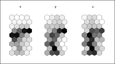
: It's pretty clear from these border maps which nodes
(dark ones) lie
: between the clusters. Again, it's reasonably easy to visually pick
out
: the clusters here. In the x-map, we see strong evidence of two clusters
: (which we know to be cluster 1 and 3). In the y- and z-maps, we see
: the strong distinction among three different clusters (although the
: separation between cluster 3 and 1 is weaker than between 2 and 3).
: Primary Component Analysis :
: By using the two largest eigenvectors of the data set,
we can construct a
: basis upon which to project the map nodes. For some types of clustering
: (not sure what kinds yet, give me more time to tinker), this method
: reveals the number of clusters very well, and relatively how each
dimension
: contributes. I've yet to figure out a way to quantitatively prove
the number
: of clusters.
: >> [Pd,V,me] = pcaproj(D.data,2); %project data
into PCA comps
: >> Pm = pcaproj(sMap.codebook,V,me); %project the prototypes
: >> colormap(gray);
: >> for i=1:3 %display PC1 vs PC2 projections
: >> subplot(2,2,i), cla, hold on
: >> som_grid('rect',[size(data,1) 1],'coord',Pd,'Line','none',...
: >> 'MarkerColor', som_normcolor(D.data(:,i)));
: >> hold off, title(D.comp_names{i}) xlabel('PC 1'), ylabel('PC
2');
: >> end

som_PCprojections.gif
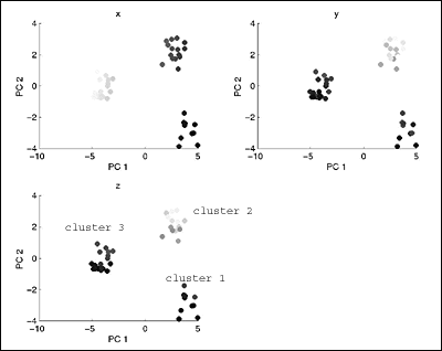
: Again, we can very clearly see the three clusters (labeled
accordingly) in the
: data set.
: Conclusions :
: The SOM Toolbox is a truly excellent piece of free software.
While it does
: require a MatLab license, if you're serious about data modelling and
: classification (which really extends to just about all statistical
fields), then
: the SOM Toolbox will do you right.
: Disadvantages
: 1. difficult to automate analysis (related to geometry of SOMs)
: 2. very sensitive to data normalization
: Advantages
: 1. allows cluster analysis of high dimensional data sets
: 2. superb visualization techniques
: 3. clear documentation of primary methods
: Even more advanced analysis (coming soon)
: Reference and Resources :
: SOM Toolbox homepage
: http://www.cis.hut.fi/projects/somtoolbox/
: Dr. Teuvo Kohonen's homepage
: http://www.cis.hut.fi/teuvo/
: SOMs in action - Dr. Samuel Kaski's homepage
: http://www.cis.hut.fi/sami/
: Explanation of Self-Organizing Map algorithm
: http://davis.wpi.edu/~matt/courses/soms/#Main
Algo
: Growing Neural Gas Demo (Java)
: http://www.neuroinformatik.ruhr-uni-bochum.de/ini/VDM/research/gsn/DemoGNG/GNG.html
|

